Effects of Non-uniform Heat Transfer in a Tempering Process on Glass Quality

First presented at GPD 2017

Abstract

Importance of heat transfer control on created residual stresses is well-known. Tempering of thin glasses has given new challenges not only to uniformity of heat transfer but also to energy consumption because very high heat transfer coefficients are required. Cooling is achieved by using arrays of high velocity small air jets located near the glass surface which create large variation of the local heat transfer coefficient. Simultaneously optical anisotropies which are seen as stripes or spots in glass panes are formed.

These cannot be avoided in all light and viewing conditions even if cooling is uniform, but non-uniformity surely increases the effect. In this paper numerically calculated (CFD) local heat transfer results of impinging jets are presented and used as an input in the numerical modeling of residual stresses. Simple validation cases are presented for both the heat transfer and residual stresses. The solved residual stress distributions are then compared to anisotropy distributions of tempered glass panes with a plane polariscope.

Introduction

In the glass tempering process heat transfer is the basis of the process. Glass is first heated above 600 °C and then cooled down below 450 °C in a couple of seconds to cause residual stresses to form in the glass. A stress profile where surface is under compression and mid-region is under tensile stress is formed. The temperature of the glass must be raised to a suitable level before cooling. Too hot temperature can cause roller waves or other local bending faults. Too low temperature prevents residual stresses from forming [1]. Uneven temperature field can cause different bending faults or give uneven stress distribution over area.

The cooling rate must be high in order to cool down the glass fast enough to produce a sufficient residual stress level. In order to produce visually pleasant glass the cooling must also be uniform enough. Natural light from clear blue sky or from a reflection can be polarized and expose the uneven quality of the glass as visual defects called anisotropy. In industrial setting the inspection of glass panes can be done by using a plane polariscope [2].

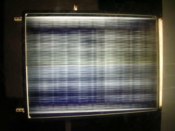
Fig.1 shows extreme optical anisotropies of a tempered glass plate, less obvious patterns like this can be seen in car rear-windows with polarized sun glasses. They are caused by a stationary cooling jet arrangement.

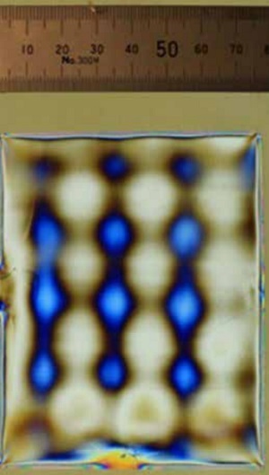
An example of normal tempered glass that was quenched while moving, is shown in Fig. 2. It is well known that uneven heat transfer causes uneven residual stresses, which in turn cause anisotropy.

The details of the mechanism are, however, not well studied. Depending on the level of anisotropy the visual quality of the tempered glass can be kept good or bad. Also the location of glazing and amount of polarized light in that area affects the level visual defects [2].

In a tempering process the cooling nozzle system can consists of thousands of jets, which should be located in such a way that relatively uniform heat transfer over the surface area is obtained. However, the highest heat transfer is at the jet stagnation point area and it decreases when the distance from the stagnation point increases [3].

During cooling the glass moves first from the heating section to a cooling part, where the local heat transfer at each point of glass surface is changing over the time. This position change relative to nozzles makes heat transfer more uniform over the area and time.

Due to movement, the local stress does not change significantly in the glass movement direction. However, the stresses perpendicular to the glass moving direction changes due to the differences in local heat transfer. This non-uniformity of forced convection in quenching causes stripes in the glass movement direction.

Uniform stress distribution is especially important in glasses which are made to be placed in architecturally important buildings, because polarized light occurs in normal daylight.

In this paper local heat transfer of impinging small jets on surface heat transfer and residual stresses is studied. Convection heat transfer results are calculated using the open source CFD software OpenFOAM. Temperature distribution in a glass and residual stresses are calculated using FEM in the Ansys software. Calculated heat transfer results are compared to measured results of a single jet in order to check the validity of modelling. Numerically obtained convective heat transfer coefficients are used in the modelling of a real tempering line with different jet arrangements. At the end, distributions of residual stresses are compared to anisotropy patterns of tempered glass panes measured with a plane polariscope.

2 Heat transfer

In order to solve the residual stress distribution in a glass plate a temperature distribution of the plate must first be solved. The glass is assumed to have a constant initial temperature before cooling. Only the calculation of cooling in a tempering process is dealt in this paper. The solution of cooling consists of two parts: heat conduction inside the glass and heat convection from the glass surface to air. Both are solved using numerical methods and include the local and temporal variation of heat transfer.

2.1 Conduction in glass plate

Temperature distribution and history in the glass plate with no internal sources is obtained from the following equation

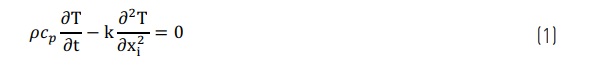
where the thermal properties of glass, i.e. density ρ, specific heat cp and thermal conductivity k, are temperature-dependent and isotropic. The effect of radiation in Eq.1 during cooling is very small and it is ignored. In order to solve the above heat conduction equation it is necessary to first solve the convective heat transfer coefficient from the glass surface by assuming that the heat transfer coefficient and glass surface temperature are not coupled together

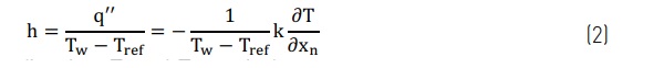
where xn is the surface normal direction, Tw and Tref are is the surface and cooling air temperatures. The heat transfer coefficient, Eq. (2), provides a boundary condition for Eq. (1) and is solved using the k-ω-SST turbulence model considered in the next section. Eq. (1) is solved using FEM of the Ansys 17 code [4]. The heat wall heat flux is solved from the energy equation in the CFD model, see next section.

2.2 Convection in glass-air interface

Convection is solved with the Finite Volume Method using the open source software OpenFOAM [5]. The validity of calculation is tested by comparing results to experimental data of a single jet in Fig. 3b.

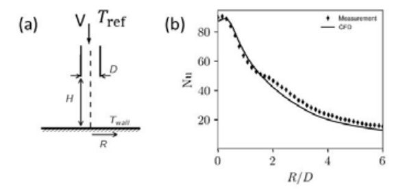
The test case was chosen from Alimohammadi’s paper [6] with Re=14000, H/D=4, and D=13mm. The Nusselt number Nu=hD/ka, where h is the convective heat transfer coefficient, D is the nozzle diameter and ka is the thermal conductivity of air. Results and schematic figure of nozzle-plate system are given in Fig. 3.

The nozzle height to nozzle diameter ratio H/D agrees well to the one used in tempering. The Reynolds number Re = VD/v, where V is the flow speed, D is the nozzle diameter and is the kinematic viscosity of air, is roughly half of the one used in the tempering process. It can be seen that CFD predicts the heat transfer with good accuracy. All predicted Nusselt number fall within 15% range of the measured ones.

The convection results used in this paper for the residual stress modeling are produced using a 3D model. The cooling section jet array is made of repeating structures and only one of these structures needs to be included into calculations.

The glass surface is at a constant temperature of 500 °C roughly corresponding to the mean of the relevant glass temperature range for tempering. No wall functions are used for the glass surface because wall functions are not suitable for impinging jet flows.

Navier-Stokes equations for steady-state compressible flow are solved using Reynolds averaging for turbulence. Menter’s k-ω-SST [7] model for turbulent kinetic energy is used

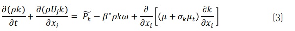
and specific dissipation is solved from the equation

The model used in OpenFoam 4.0 [5] differs in detail from the one proposed by Menter [7]. Details are given in the the OpenFoam source code or in the paper by Mikkonen and Karvinen [8]. Ideal gas law is used as the equation of state and Sutherland’s correlation is used for viscosity to include the effect of temperature. Heat convection at the glass surface is very sensitive to grid size and quality. A very fine grid size is used near the glass surface. Grid independency is studied by repeatedly refining the mesh. For a 3D calculation millions of cells are needed. For an introduction to impinging jet heat transfer, see the paper by Zuckerman and Lior [9].

3 Residual stress

The calculation of residual stresses due to tempering process is based on the thermo-mechanical model. For thermal stresses the temperature distribution has to be solved using the theory shown above in Chapter 2.1. The mechanical behavior of the glass during the cooling process based on the thermal strains and the viscoelastic behavior of the glass at different temperatures. The stress of the glass at each time can be calculated by using Eq. (5) [10].

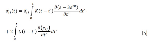
Where σij is the directional stress, K(t) is the bulk relaxation modulus as shown in Eq. (6), G(t) is the shear relaxation modulus as shown in Eq. (7), and are the strain components as shown in Eqs. (8) and (9) and is the thermal strain as shown in Eq. (10). In the mechanical model the temperature-dependent viscoelasticity and the structural relaxation are taken in consider [11].

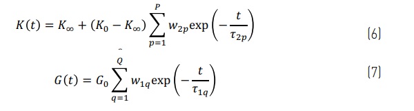
where subscript 0 is the initial value and ∞ is the value at infinite time. In the weighting factors w and relaxation times τ the subscript 1 is for the shear relaxation and 2 for the bulk relaxation.

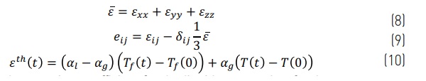
where αl is the thermal expansion coefficient for the liquid state and αg for the glassy state. Fictive temperature Tf is related to structural relaxation of glass [11]. A detailed theory of the model is in the literature [12].

In calculations Ansys 17.0 software is used [4], which is based on Finite Element Method (FEM). The calculation has to be done transient using different time steps over the whole cooling time to solve the residual stress. The model verification has been done in the thesis by Aronen [12] and compared to experimental results by Gardon [13], see Fig. 4, which both were obtained using uniform heat transfer coefficients over the area.

Modeling results are the same as experimental results with low heat transfer coefficients, but with high heat transfer coefficients the modeling results are about 10 % lower compared to experimental results. It can be noted that internal stress measurements are not easy they can contain errors.

4 Anisotropy

The effect of the anisotropy can be explained with the principal stress differences. The photoelasticity is used to determine the stress field in transparent materials with an experimental method. In the stress-optic law the principal refractive indices are expressed as a function of principal stresses. The refractive index in direction 1 is presented in the Eq. (11). The equations in other directions are the same except for the subscripts in labeling [14].

Parameter n0 is the refractive index of unstressed material and constants C1 and C2 are depending on material. For the plane stress the normal to plate stress σ3 = 0 and the light is passed through the plate in the direction 3. Then the stress difference σ1- σ2 is studied. The relative retardation δ is presented by the equation of Wertheim law and it is [14] Where C=C1-C2 is photoelastic constant and d is the thickness of material. In the case that stress distribution is changing over the thickness the relative retardation can be integrated over the area [14].

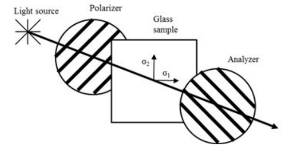
The plane polariscope, as presented in the Fig. 5, can be used to see the colorful anisotropy pattern. In the plane polariscope light is first polarized at the polarization filter. Polarized light passes through the glass with residual stresses where the relative phase shift of components of polarized light forms. Finally when polarized light with relative phase shift passes through the second polarization filter, which is rotated 90° comparing to the first filter.

5 Computational and experimental results of tempered glass

5.1 Convective heat transfer in tempering

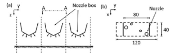
Using the nozzle geometry used in glass tempering machine cooling section, see Fig. 6, the heat transfer coefficients are calculated. The overpressure is 5000 Pa compared to the outside atmosphere pressure and jet velocity about V ≈ 100 m/s, H/D ≈ 4, and D ≈ 5 mm. The used numerical methods are described in section 2.2 and expect for the geometry and over pressure are the same as used in the validation case in Fig. 3. The total length of a nozzle plate is 80 mm and plates are installed 120 mm apart from each other.

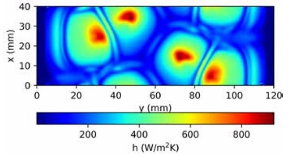
In Fig. 7 calculated heat transfer coefficient in the glass surface is shown. It can be seen that heat transfer of a nozzle array is qualitatively similar to heat transfer of a single nozzle shown in Fig. 3. Heat transfer is highest near the stagnation point where the jet hits the wall directly and decreases with increasing distance from the stagnation point.

Heat transfer coefficients in Fig. 7 are used to calculate the temperature field for a moving glass, when the effect of jet locations is studied below. Under the supporting rollers, near the edges of the calculation domain in the y-direction, heat transfer is small because of near zero air velocities. The irregularities in the fields are caused by the transient nature of jets.

5.2 Residual stress distribution in glass

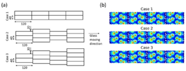
The stress distribution in glass after tempering process is calculated by using the convective heat transfer coefficient distribution solved above and shown in Fig. 7. The stress distribution has been solved for three different cases. In the first case (C1) the solved local heat transfer distribution repeats periodically. In the second case (C2) heat transfer distributions in sequential periods are shifted in the x-direction by the half width of the periodical distance. In the third case (C3) sequential periods are shifted in the x-direction by the quarter of the width. Illustration of these cases is shown in Fig. 8. The width of sequential period is 40 mm and length is 120 mm.

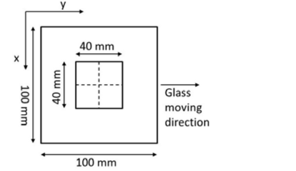
In the modelling the 3.85 mm thick glass moves relative to the quenching system continuously in one direction (y-direction) for 5 seconds with the speed of 450 mm/s. This corresponds approx. glass movement in a 2 m long chiller. After 5 seconds the cooling has changed to a uniform heat transfer coefficient (330 W/m2K) cooling and glass movement is stopped. Then glass is cooled close to room temperature. The change to uniform heat transfer coefficient is done to simplify the calculation. The beginning of the cooling is the most important and the change after 5 seconds does not effect on the residual stress distribution. Heat transfer is symmetric relative to the mid-plane. The size of modeled area, where residual stresses are considered, is 100 x 100 mm2 as shown in Fig. 9. 

The initial temperature of the glass is 650 °C. 

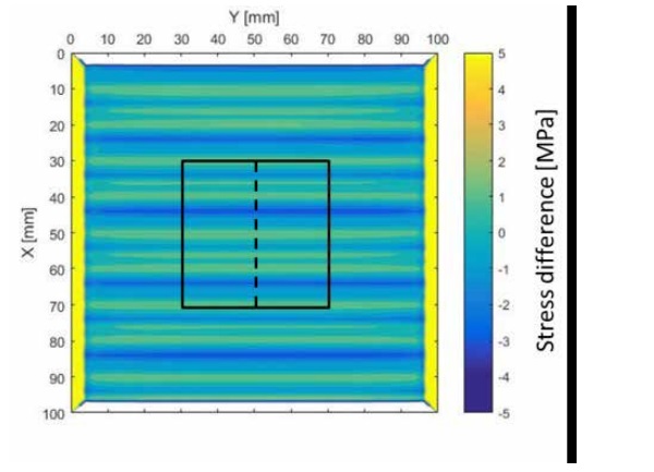
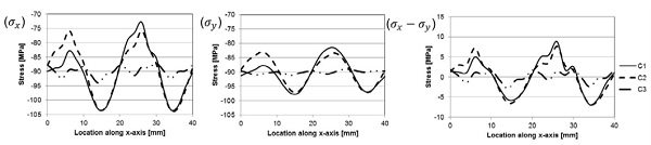
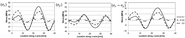
The material properties for glass used in the model are the same as used by Aronen [12]. The results show that the stress in 40 x 40 mm2 size area in the center of modeled area varies significantly only in the x-direction, as shown in Fig. 10. The stress variations are due to the local variations in average heat transfer. The stress in the x-direction and the y-direction as also the stress difference along the x-direction with different nozzle systems at the surface and in the mid-plane are shown in the Figs 11 (surface) and 12 (mid-plane). These stresses are plotted along the dashed line shown in Fig. 10. Results show the clear influence of the shifting of the nozzle plates to uniform the local heat transfer and stress distribution.

Results for Cases 1 and 2 can vary over 20 MPa between maximum and minimum stress in surface and 10 MPa at mid-plane. Case 3 is more uniform and the stress difference between maximum and minimum values is less than 5 MPa.

5.3 Anisotropy observations in tempered glass

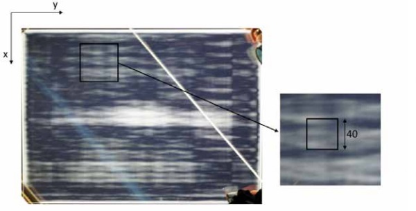
The modeled stress results are compared to real anisotropy distribution from a test sample shown in Fig. 13. In the experiment test sample of clear float glass with the size 585 x 800 mm2 and the thickness 3.85 mm was tempered. Glass was first heated to about 630 °C and the cooled with nozzle cooling system similar to Case 3 in numerical results.

The overpressure in a n air box was 5000 Pa and distance from nozzle to plate was 16 mm. In the cooling part, glass was moving with speed 450 mm/s. The stress on the surface was measured with the GASP surface stress polarimeter. Depending on the location stress was between 89-93 MPa. The visual anisotropy in the test sample is shown in Fig. 13.

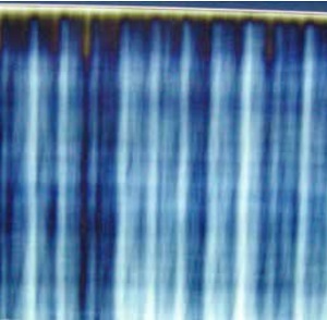
For the anisotropy distribution the polarization filters and the glass sample are oriented as in the Fig. 10 In Fig. 13, the main result to compare the numerical results and experimental results is the horizontal wide stripes which repeat regularly. In the enlarged area in Fig. 13 three regularly repeating horizontal stripes are shown.

The width of one strip is about 40 mm, which is same to numerical results. The stress level in the anisotropy distribution is not available. However, by comparing the intensity differences in the enlarged area in the Fig. 13 to the intensity differences in the center of pane in the Fig. 13, the stress change due to nozzle location is smaller.

6 Conclusions

Visual quality of the tempered glass without anisotropy is coming more and more important factor in tempered glass and tempering machine business. The most important factor to glass quality is the control of heat transfer, which should be uniform over the glass plate and symmetric over the mid-plane of the glass.

This paper shows that with state-of-theart CFD numerical methods it is possible to calculate the heat transfer during quenching. These heat transfer result can be used in FEM program to solve the residual stresses caused by the heat transfer.

By comparing calculated residual stress distributions and visual observations of tempered glass with a plane polariscope similarities can be noted. With numerical methods the effect of the nozzle placements on stress distribution can be studied and optimized. Though, the modeling and experimental results of residual stresses show similar behavior as anisotropy in tempered glass the stress level cannot be solved from anisotropy image.

References

[1] Aronen, A. Karvinen, R., Effect of initial temperature and cooling rate on residual stresses of tempered glass, Glass Structures & Engineering, under review.

[2] Illguth, M., Schuler, C., Bucak, Ö., The Effect of Optical Anisotropies on Building Glass Façades and its Measurement Methods, Frontiers of Architectural Research, Vol. 4, pp. 119-126, 2015.

[3] Holger, M., Heat and Mass Transfer between Impinging Gas Jets and Solid Surfaces, Advances in Heat Transfer, vol. 13, pp. 1-60, 1977.

[4] ANSYS® Academic Research, Release 17.0

[5] The OpenFOAM foundation, http://www.openfoam.org/, version 4.0, 2017.

[6] Alimohammadi, S., Murray, D., Persoons, T. Experimental Validation of a Computational Fluid Dynamics Methodology for Transitional Flow Heat Transfer Characteristics of a Steady Impinging Jet, ASME. Journal of Heat Transfer, Vol. 136, 2014

[7] Menter, F. R., Kuntz, M., Langtry, R., Ten Years of Industrial Experience with the SST Turbulence Model, Turbulence, Heat and Mass Transfer, Vol. 4, pp.625 – 632, 2003.

[8] Mikkonen, A., Karvinen, R., Heat Transfer of Impinging Jet: Effect of Compressibility and Turbulent Kinetic Energy Production, IX International Conference on Computational Heat and Mass Transfer, 23-26 May 2016 Cracow, Poland, 2016.

[9] Zuckerman, N., Lior, N., Jet Impingement Heat Transfer: Physics, Correlations, and Numerical Modeling, Advances in Heat Transfer, Vol. 39, pp.565–631, 2006

[10] Flügge, W., Viscoelasticity, 2nd ed., SpringerVerlag, Berlin, Germany, 1975.

[11] Scherer, G., Relaxation in Glass and Composites, John Wiley & Sons, Inc., USA, 1986.

[12] Aronen, A., Modelling of Deformations and Stresses in Glass Tempering, Dissertation, Tampere University of Technology, 2013.

[13] Gardon, R., The Tempering of Flat Glass by Forced Convection, Proceedings VIIth International Congress on Glass, Brussels, Belgium, 1965.

[14] Aben, H., Guillemet, C., Photoelasticity of Glass, Springer-Verlag, Germany, 1993.

Acknowledgement

The authors acknowledge the Finnish Funding Agency for Technology and Innovation (Tekes) for partly funding this work during the program Energy Efficient Tempering of Thin Glasses for Solar Energy Next Generation Products. The authors also acknowledge the University of Sydney HPC service at The University of Sydney for providing HPC and software resources that have contributed to the research results reported within this paper.