Authors: S. Dix, P. Müller, C. Schuler, S. Kolling & J. Schneider
Source: Glass Structures & Engineering | https://doi.org/10.1007/s40940-020-00145-3
Abstract
In the present paper, optical anisotropy effects in architectural glass are evaluated using digital image processing. Hereby, thermally toughened glass panes were analyzed quantitatively using a circular polariscope. Glass subjected to externally applied stresses or residual stresses becomes birefringent. Polarized light on birefringent materials causes interference colors (iridescence), referred to as anisotropies, which affect the optical appearance of glass panes in building envelopes. Thermally toughened glass, such as toughened safety glass or heat strengthened glass, show these iridescences due to thermally induced residual stress differences.
RGB-photoelastic full-field methods allow the quantitative measurement of anisotropies, since the occurring interference colors are related to the measured retardation values. By calibrating the circular polariscope, retardation images of thermally toughened glass panes are generated from non-directional isochromatic images using computer algorithms. The analysis of the retardation images and the evaluation of the anisotropy quality of the glass is of great interest in order to detect and sort out very low quality glass panes directly in the production process.
Therefore, in this paper retardation images are acquired from different thermally toughened glass panes then different image processing methods are presented and applied. It is shown that a general definition of exclusion zones, e.g. near edges is required prior to the evaluation. In parallel, the limitations in the application of first-order statistical and threshold methods are presented. The intend of the investigation is the extension of the texture analysis based on the generation of Grey Level Co-occurrence Matrices, where the spatial arrangement of the retardation values is considered in the evaluation.
For the first time, the results of textural features of different glass pane formats could be compared using reference areas and geometry factors. By reduction of the original image size, the computation time of textural analysis algorithms could be remarkably speeded up, while the textural features remained the same. Finally, the knowledge gained from these investigations is used to determine uniform texture features, which also includes the pattern of anisotropy effects in the evaluation of thermally toughened glass. Together with a global evaluation criterion this can now be implemented in commercial anisotropy measurement systems for quality control of tempered architectural glass.
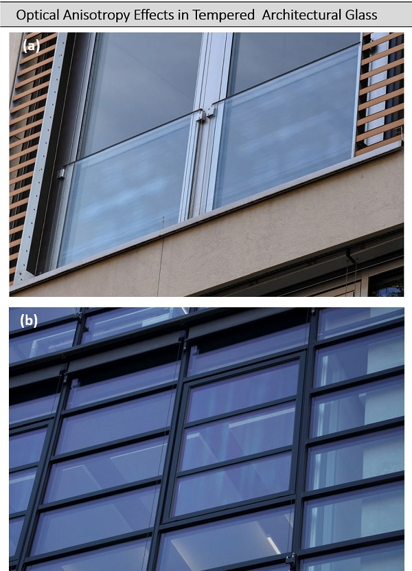
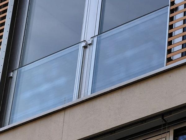
Thermally toughened glass is often used in architecturally ambitious buildings because of its high strength and thermal shock resistance. The glass dimensions required for high-quality façade projects can only be achieved sensibly with thermally toughened glass due to technical, economic and safety-related boundary conditions (fracture behavior). However, with this type of glass, optical phenomena can occur that can be perceived as disturbing by the observer. The so-called anisotropies or iridescence can become visible as a characteristic pattern in the façade in the form of grey, white or rainbow-colored spots, rings or stripes under certain light incidence, weather conditions and daytimes, see Fig. 1.
The cause of these phenomena is based on the manufacturing process of the glass panes and the perception of the human observer under polarized light, c.f. Illguth et al. (2015).The thermal tempering of glass is an established process in which the basis glass is heated in a tempering furnace to about 100K above the glass transition temperature Tg and then rapidly cooled by quenching with air. This leads to the formation of residual stresses, characteristic of thermally toughened glass. The widely used horizontal tempering process is influenced by heat transfer and glass support and is part of work by Mikkonen et al. (2017), Pourmoghaddam and Schneider (2018), Karvinen and Aronen (2019).
Due to local temperature gradients in the heating and cooling process of the glass, differences in the principal stresses can occur (Nielsen et al. 2010). Even minimal differences lead to a change in the optical properties of the glass. An otherwise optically isotropic medium becomes a birefringent medium with direction-dependent optical (anisotropic) properties. Anisotropy effects are seen as undesirable (Pasetto 2014), but they are not considered as defects or deficiencies according to the current standards (EN 12150 2015; EN 1863 2012; ASTM C 1048 2018).
The colored iridescence effects can be explained with the help of the photoelasticity. Fundamentals can be found in Brewster (1815), Frocht (1948), Kuske and Robertson (1974), Dally and Riley (1978). When a polarized light beam enters a flat glass, it is split in two directions parallel to the principal stresses. If these principal stresses are not equal, the two partial rays propagate at different velocities in the glass, resulting in a path difference after the light rays leave the glass. The path difference is also called the retardation. Since the human eye perceives the retardation of polarized daylight as interference colors (Sørensen 2013), this is directly related to visible anisotropy effects. By varying the retardations over the area of the glass pane, the typical anisotropy effect images as shown in Fig. 1 are obtained. Depending on the level of the retardations, weakly perceptible black and white patterns or strongly visible colored patterns will result.
In Illguth et al. (2015) a measuring method based on the RGB-photoelasticity by Ajovalasit et al. (1995) was tested, allowing the quantification of full field retardation images on thermally toughened glass panes. Since then the use of this technique has been further developed and a series of measurements have been performed in Dix and Schuler (2018), FKG (2019). In these investigations first dependencies in the generation of anisotropy effects in thermally toughened glass (e.g. influence of glass thickness, differences between clear and coated glass) could already be determined. Although a large number of offline and inline measuring devices have now been developed, the final evaluation of retardation images remains still unresolved. Currently, evaluation methods are used that follow global approaches and thus do not take into account the spatial relationship, such as patterns and local characteristics. Thus, completely different pattern phenomena can have a divergent effect on the observer even with the same global characteristic values.
Digital image processing methods offer far more tools to evaluate the retardation images. Besides newer pattern recognition techniques, such as segmentation approaches and neural networks, Hidalgo and Elstner (2018) have applied common texture analysis algorithms (Haralick et al. 1973) to retardation images of equal size for the first time. Through the formation of Grey-Level-Co-occurrence Matrices (Gonzalez et al. 2011) the spatial arrangement of retardation values is determined and evaluated by textural features. However, it is still unclear whether and how the transferability to glass panes of different sizes can be achieved and whether the time-consuming calculation of the algorithms for an application in online measuring systems can be reduced. The intention of the investigations is therefore to find a method to evaluate spatial patterns of the anisotropy effects of thermally toughened glass independent of the glass geometry before installation in the façade, during glass production.
Experimental investigations
Setup for photoelastic measurements
In the present work, different digital image processing methods are applied to retardation images of thermally toughened glass panes to evaluate optical anisotropy effects caused by residual stress differences. For this purpose, full-field photoelastic measurements were carried out using calibrated polariscopes according to Ajovalasit et al. (1995), Illguth et al. (2015) and Schaaf et al. (2017). Principles of photoelasticity can be found in Frocht (1948), Kuske and Robertson (1974), Dally and Riley (1978). An overview of further photoelastic techniques can be taken from Fernández et al. (2010) or Ramesh and Ramakrishnan (2016).
The acquired images of a circular polariscope are also called isochromatic images because they are rotationally invariant due to the circular polarization of the emitted light beam. Detailed information on the occurrence of retardation s in the circular polariscope and its connection to the interference colors can be found in Illguth et al. (2015) and Schaaf et al. (2017). Under the assumption that the photoelastic constant C does not vary over the glass thickness t, the retardation s is determined by the integral of the principal stress difference σ1−σ2 and can be expressed mathematically by:
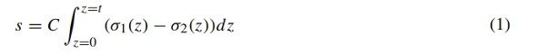
In the framework of these investigations the two following research-based circular polariscopes were used, see Fig. 2.
In Setup A, isochromatic images of small glass panes with a size of up to 1.0 x 1.1 m2 can be acquired by using a conventional digital camera with a left circular polarizing filter and a white light source equipped with a right circular polarizing filter. The white light source of the manufacturer WRG consists of a two-dimensional illuminating box with high-frequency daylight and a color temperature of 6500K. For the determination of retardations out of the isochromatic images it is necessary that all parameters regarding the exposure and image quality shall remain constant for a calibrated system. This implies that it is important to keep the exposure time, aperture, white balance and sensitivity of the sensors constant.
With setup B it is possible to acquire images of glass panes with a width of 2.0 m and theoretically unlimited length. However, in this case the images are taken with a line scan camera. To achieve a complete image of a pane, the pane must be moved through the line scanner. This has the advantage that larger dimensions of glass panes can be scanned without the need for light sources with polarized light in the dimensions of the glass. Therefore, we use a setup with a commercial line-scan camera Dalsa Spyder3 Color (SC-34-02K80) with 2048 pixels in width and a common white LED bar light from smart vision lights LX300-WHI-L with a color temperature of 6500K. The configuration of the camera with its photometric parameters (exposure time, etc.) is performed here in the software interface of the camera.
This is another great advantage to Setup A, because it allows a direct output and further processing of the polarization filter images. Identical to Setup A, Setup B also uses circular polarizers as polarizers in front of the light source and as analyzers with a 90∘∘ rotated retarder in front of the camera. The circular polarizing filter CP42HE of the manufacturer ITOS was chosen because of its high transmission in direction of polarization and a good blocking of the other directions for a large spectral bandwidth. Setup A leads to an image resolution of 0.5 mm/px and Setup B to 1 mm/px. Both resolutions seems to be high enough, if one considers the typical patterns of anisotropies in Fig. 1. The generated polarizing filter images of the glass panes are evaluated by an algorithm that assigns the corresponding retardation to each pixel, see Sect. 2.2.
Analysis algorithm
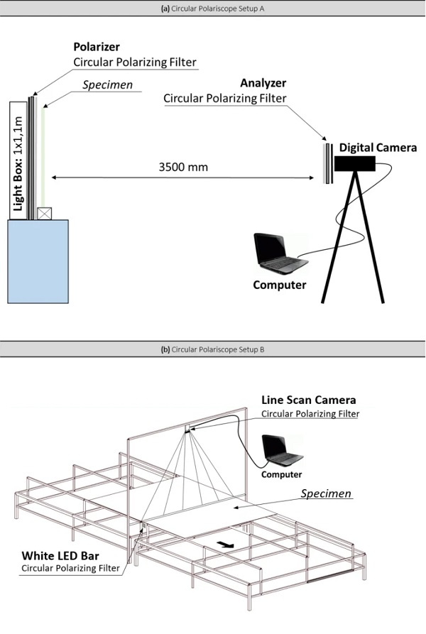
In order to allow a correlation between the color of the isochromatic images (RGB intensities) and the optical retardation s, a calibration chart for each polariscope will be generated first. As mentioned in Sect. 2.1 the photometric parameters and polariscope equipment must be identical during image acquisition for the calibration chart and for the tempered glass samples under investigation. Conversely, separate calibration charts must be created for different camera sensors, light sources or when analyzing coated glass.
The basic method for the determination of retardation images using calibrated polariscopes was presented in detail in Illguth et al. (2015) and Schaaf et al. (2017). The generation of a calibration chart starts with the insertion of a Babinet-Soleil compensator into the beam path between camera and light source. This optical device can be used for a wide range of wavelengths and the desired retardation can be continuously adjusted. Calibration chart images for the investigations were taken in steps of 10 nm phase shift. The RGB intensities of the resulting image series are then compared with the retardation in an algorithm routine and intermediate values are interpolated in steps of 1 nm. Calibration runs with intermediate steps of 1 nm phase shifts were also carried out in own studies. A significant increase in accuracy by increasing the intermediate steps in the calibration could not be determined.
In Fig. 3 a the calibration chart with representative spectral color of Setup A is shown. This is similar to the analytically calculated Michel-Lévy interference color chart from Illguth et al. (2015), which represents the relationship between retardation s and the interference color sensitivity of the human eye. Interference colors from anisotropes such as Fig. 1 can therefore be reproduced with RGB-photoelasticity. Comparing the spectral colors of the calibration chart with the isochromatic image in the circular polariscope Fig. 3b, the subjective observer can already guess that the dark areas are below 50 nm and the bright white areas indicate a retardation around 200 nm.
A retardation value at each pixel of an isochromatic image can now be determined with the aid of evaluation software. During evaluation, the search algorithm compares each pixel of the image (Rp,Gp,Bp) with that of the calibration chart (Ri,Gi,Bi). Here the best fit with minimization of the error sum E is calculated according to:
![]()
The generated retardation images can then be visualized in 2D or 3D false color plots, see Fig. 3 c. The five-color scale in nm allows the observer to quickly locate areas with high retardations in detail. The sequence of the measurement method is summarized in Fig. 3.
Retardation measurements
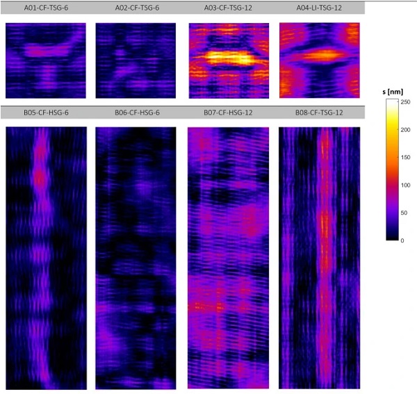
For the purpose of this investigation, eight tempered glass panes of different size (length l, width w), thickness (t), glass type (gt) and prestressing level (pl) were measured. The dimensions given are nominal values. The raw glass panes of clear float (CF) and low iron (LI) originate from the same float glass manufacturer. They were further processed by different glass processors into heat-strengthened glass (HSG) and toughened safety glass (TSG) to obtain different anisotropy patterns. Information of the samples are summarized in Table 1. In Fig. 4 the acquired retardation images of the glass samples in 2-D false color plots are shown.
Table 1 Information on the used thermally toughened glass samples - Full size table
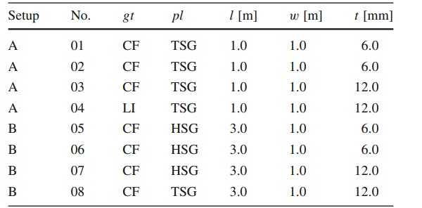
With the help of the colored scale, the occurring retardations can be perceived in more detail. Here it is shown that for each glass pane, different levels of retardation and differing pattern characteristics across the glass area result. Since the retardation s according to Eq. (1) is summed over the integral of the thickness t, thicker glass panes also show more areas with high retardations. The patterns are diverse, ranging from partly spotted to striped patterns. In the following, an image processing method is sought which can classify the samples into good and low quality glass panes based on the frequency of high retardations and the conspicuity of patterns.
Methods of digital image processing
Statistical methods
Statistical methods are the first step in evaluating quantitative information. The information, in this case retardation values per pixel, can be processed in grey values of 8 or 16 bit (0–255, or 0–65,535 numerical values) depending on the level of retardation. To ensure that higher retardation values are not cropped at 255, the data acquisition in setups A and B (see Sect. 2.1) is performed in 16-bit data format. With the help of histograms, the frequency distribution of the grey value intensities occurring in the image can be easily visualized. Since no values above 255 nm were found in the samples from Sect. 2.3, data processing in MATLAB® was carried out in 8-bit format.
First-order statistical methods have proven to be effective for quick and simple determination of comparable characteristic values from the empirical distribution of intensity values in the retardation image. The empirical distribution function depicts these values in a diagram which is the basis for our statistical analysis, see Fig. 5c. All values of the image are listed from zero to the largest retardation value along the x-axis. The y-axis shows the sum of the relative frequencies of the individual values. In engineering, αα-quantiles, such as the 5% fractile value, are often used and well known for the evaluation of test series. An α-quantile splits data into the parts α∗100% and (1−α)∗100%. Assuming that the 60% quantile is being searched for, the characteristic xα can be found in which at least 60% of the characteristic values are smaller than or equal to xα and at least 40% of the characteristic values are larger than xα.
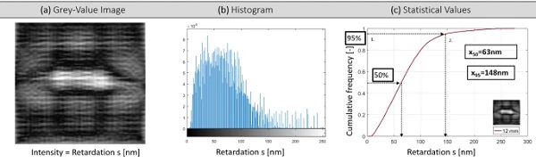
In the investigation in Sect. 4 the 95% quantile x0,95 was used under the assumption of normal distribution. The calculation of the quantile values can be expressed mathematically for k=n⋅α in integers and n number of occurring pixels as:

Threshold methods
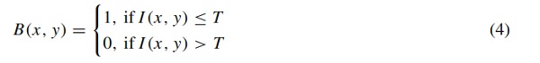
Threshold methods are common image processing tools and belong to a group of algorithms that are mainly used for segmentation of digital images. Using thresholding, the source image (grey-value image) is converted into a binary image, returned as an m-by-n logical matrix, see Gonzalez et al. (2011). Threshold methods can be implemented quickly due to their simplicity and segmentation results can be calculated with little effort. Furthermore, they offer the possibility to integrate human-subjective perception thresholds into the evaluation.
Threshold methods can be divided into global, local and hybrid threshold techniques. The more complex techniques are mainly used for medical image segmentation or document image analysis, c.f. Gatos (2014). The simplest thresholding method replace each pixel in an image with a black pixel if the image intensity is less or equal than some fixed constant T, or a white pixel if the image intensity is greater than that constant. If I(x, y) is the original greyscale image, then the resulting binary image B(x, y) is defined as:
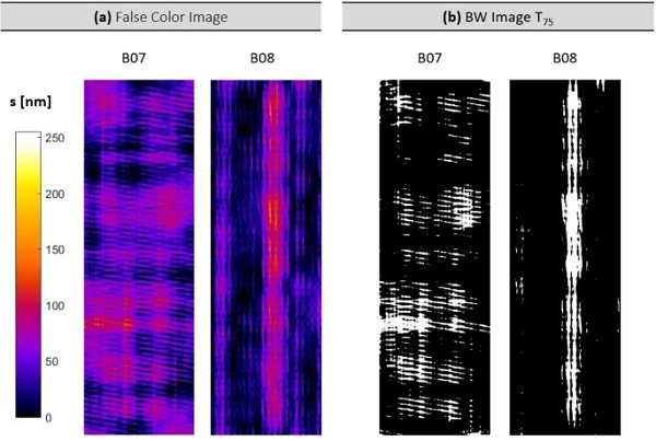
In Fig. 6b the application of a threshold of T= 75 nm is applied to the retardation images of samples B07 and B08. From the binary images, see Fig. 6b, the ratio of white pixels NI,white to black pixels NI,black can be calculated. This ratio value is also called isotropy value IsoT and can be described as:

However, it should be questioned how the value is defined by the choice of the threshold value T and whether only the isochromatic image was defined as the basis for the evaluation. In Dehner and Schweitzer (2015) the orientation of the principal stress directions is also taken into account when determining the isotropy value. Orientation was not considered in this investigation as it cannot be recorded with the methods used in Sect. 2.1. By defining multiple thresholds, different binary images and isotropy values can be output. Thresholds can also be the basis for the use of other image processing methods.
Texture analysis
Texture analysis with the determination of textural features according to Haralick et al. (1973) is a method for the recognition and evaluation of striking objects and regions of interest in images. This technique has been used successfully for years in the evaluation of medical images or remote sensing images, c.f. Soh and Tsatsoulis (1999), Aborisade et al. (2014). Hidalgo and Elstner (2018) applied these methods for the first time on retardation images, acquired with setup A at the University of Applied Sciences Munich. The aim was to develop an additional evaluation criterion which, in addition to first-order statistical methods, can also take into account the homogeneity of the image over the area.
Texture analysis starts here and since this first study was promising, the applicability of these methods will be further investigated in this study. Texture analysis is also called second order statistical method, because it not only includes intensities of pixels, but also the spatial relationship of pixels for statistical analysis. The integration of the spatial component can be realized with different methods, c.f. Soh and Tsatsoulis (1999), Gonzalez et al. (2011). The use of the Grey Level Co-occurrence Matrix (GLCM) is a proven method to relate pixel intensities with neighboring pixel intensities.
When creating such matrices, parameters must be defined in advance influencing the evaluation of the textural features. Parameters required to create a GLCM are the direction θ, the step size or distance d and the number of the grey levels Ng. A GLCM P(i, j) is a matrix where n and m represent the size of the image, i and j are matrix coordinates (grey levels). I(p, q) is the intensity level of the analyzed pixel and I(p+Δx,q+Δy) is the intensity level of the neighbour pixel separated by a spatial distance d=max(|Δx|,|Δy|) in a given direction θ. Mathematically, Hidalgo and Elstner (2018) define the GLCM as:

In this paper, rotationally invariant symmetric GLCM matrices with directions of θ is 0∘, 45∘, 90∘ and 135∘ are calculated and then normalized for texture feature extraction according to Haralick. Haralick et al. (1973) has introduced 14 features, of which Hidalgo and Elstner (2018) applied two to grey value images with stored retardation values. While the feature Contrast (C) represents the amount of local grey level intensity variation in an image, the feature Cluster Prominence (CP) defines areas of constant intensity deviating from GLCM mean values. For a “constant” image, no variation, C is zero.
Contrast (C):
Cluster Prominence (CP):
with:
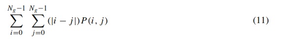
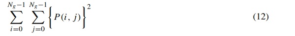
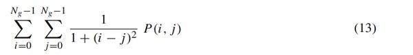
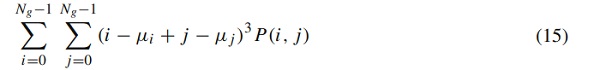
In Sect. 4.2.5 further textural features are examined according to Haralick et al. (1973), Albregtsen, F. (2008) and Aborisade et al. (2014). Thereby Eqs. (11, 12, 13, 14, 15) evaluate the homogeneity in the image. Dissimilarity is a measure of the distance between pairs of objects (pixels) in the region of interest and is similar to feature C, but here (i−j) is only included in the result on a linear basis. The Angular of Second Moment (ASM) is the most commonly used measure, which increases with less contrast in the image. The Inverse Differential Moment (IDM) also known as Local Homogeneity is also influenced by the homogeneity of the image.
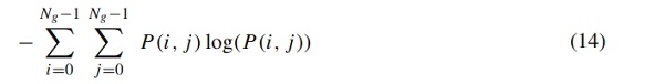
Low IDM values are indicators for inhomogenous images and high IDM values for homogenous images. Because of the weighting factor (1+(i−j)2)−1 IDM will get small contributions from inhomogeneous areas (i≠j). Entropy (ENT) is a term from information theory and is also considered a statistical measure of randomness with which the texture of an image can be characterized.
Maximum ENT is reached when all probabilities are equal. Homogeneous scenes have low ENT values, while an inhomogeneous scene has a high ENT. Like CP, Cluster Shade (CS) is an indicator of whether an image has high coherent intensities. The two differ only in the height of their exponents, see (i−μi+j−μj) of Eqs. (8, 15).
Dissimilarity (DISS):
Angular Second Moment (ASM):
Inverse Difference Moment (IDM):
Entropy (ENT):
Cluster Shade (CS):
Evaluation of the retardation images
Influence when selecting the evaluation region
In Schaaf et al. (2017) and Dix and Schuler (2018) it was shown that due to geometric constraints (e.g. edges, holes, notches and openings) areas with very high retardation occur in the isochromatic image. These unavoidable anisotropies from boundary conditions can occupy more or less large areas depending on thickness, geometry and glass type. However, a standardized definition of these zones is necessary. In the context of these investigations, zones are excluded from the assessment in accordance with the guideline to assess the visible quality of glass in buildings (Bundesverband Flachglas 2009). This guideline divides the individual glass pane into the areas rebate zone (R), edge zone (E) and main zone (M).
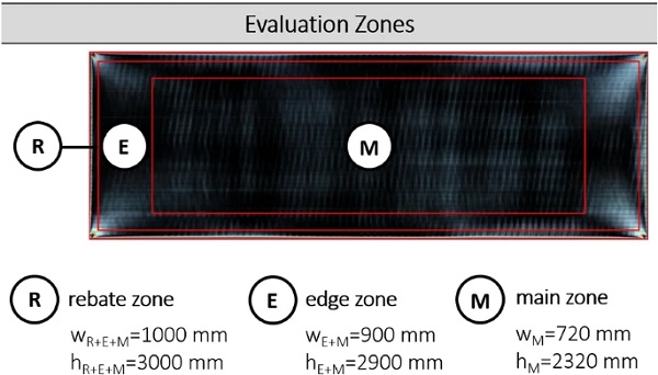
Figure 7 exemplary shows the division of the exclusion zones for the sample B07-CF-HSG-12, represented as iso-chromatic image. The geometrical influence in the boundary areas R and E is clearly visible in the form of higher retardation areas, which are represented by white to colored interference colors. The rebate zone R is defined as the visually covered area in the installed state, e.g. by cover strips, in which very high retardation far above 500 nm can occur and would falsify the evaluation. Although a thickness-dependent width R would make sense, on the one hand there are no verified measured values and on the other hand uniformly large images are required in the subsequent texture analysis.
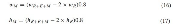
Therefore the width of the rebate zone was chosen with wR=50mm and the retardation values from this area were not considered in any evaluation. The edge zone E is the area that requires a less strict evaluation according to Bundesverband Flachglas (2009) and is declared with 20% of the respective clear width and height dimensions. The remaining main zone M is subject to the most stringent evaluation. The calculation of the width of zone MwM and the height of zone MhM is described as:
After defining the evaluation areas on the retardation images from Sect. 2.3, the image processing methods according to Sects. 3.1 and 3.2 were applied for the zones M and E + M. The effects of zoning on the results of the quantile value x0.95 and the isotropy value Iso75 at a threshold of 75 nm is compared in Table 2. In addition, the differenceΔ(E+M)−M was determined between the results of the zoning E+M and E.
Table 2 Isotropy- and 95% quantile values per exclusion zone - Full size table
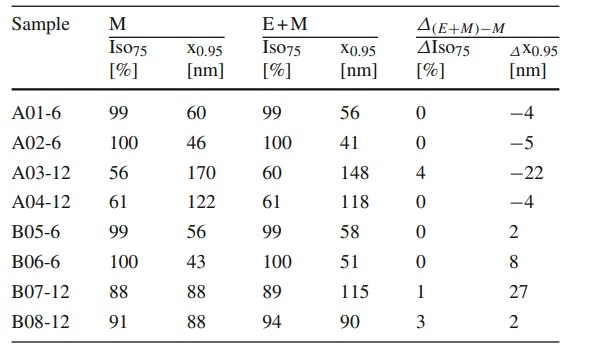
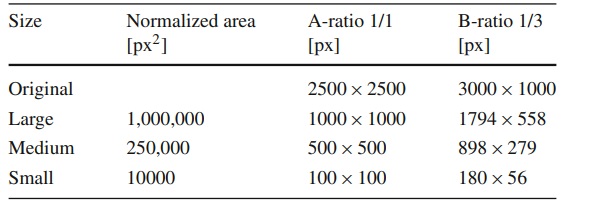
Table 3 Information on normalized area An of format A and format B - Full size table
At first it seems that the influence of zoning on the Iso 75 is only marginal (0 to 4%), whereas it is more obvious in the determination of x0.95 (−22 to 27 nm). On the one hand, this implies that when comparing different retardation images, it is essential to define evaluation zones, otherwise first-order statistical values will be distorted. On the other hand it is obvious that the isotropy value with only one threshold of 75 nm, underestimates the high retardation values in zone E. A detailed evaluation of the retardation images can be found in Sect. 4.3.
Effects which influence the texture analysis
Normalization for texture analysis
Texture analysis can be of future interest as an additional criterion for the evaluation of retardation images. In Hidalgo and Elstner (2018), this was applied to a set of retardation images corresponding to the same glass format, as mentioned in Sect. 3.3. In our study, the texture analysis approach is applied to glass panes of different sizes and format types. In addition, the retardation images from Sect. 2.3 also differ in resolution [px] because the images were acquired with different setups, see Sect. 2.1 and Table 3. The parameters for the formation of the GLCM, which are necessary for texture analysis, are described in Sect. 3.3. Based on the step size (distance d), the four directions and the symmetry condition of the GLCM, the intensity of the reference pixel i is compared with the neighboring pixels j. The area covered by these parameters will be referred to as window in the following text.
If one considers the Eq. (6), it can be seen that source images of different sizes produce different sized GLCMs. In order to achieve a scale-independent evaluation of the textural features, a normalization of the evaluated area M to a reference area An is proposed and the geometry factors fr, fI,n and fws,n are introduced. In Sect. 4.2.2 parameter studies are performed on differently sized normalized reference areas AL, AM and AS, see Fig. 8. Thus the index n represents the different sizes of the normalized reference area A. The effects of the different ratios of glass format A to B on the respective reference areas are shown in Table 3. For the normalized reference area AL this results in an image size of 1000 px × 1000 px for glass format A and an image size of 1794 px × 558 px for glass format B.
The scaling to the normalized area Ann is performed in Matlab® using the function "imresize", the interpolation method "nearest neighbor" and a scaling factor which is defined here as image scale factor fI,n. For the calculation of fI,n the ratio factor fr is determined first, which considers the ratio height to width. Both factors are mathematically expressed as:
For the calculation of the geometry factors, Eqs. (18, 19 and 20), hM,O, wM,O and wM,n in [px], as well as the true width of the zone M, wM in [mm], are used. Here h is the height of an image and w is the width of an image. The guided indices stand for M the evaluation of zone M and O for the original image size. To create comparable GLCMs, the next step is to calculate the window size factor fws,n, which can be described as:
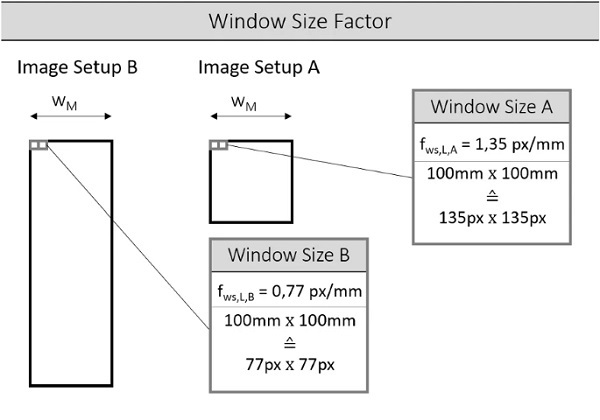
Multiplying fws,n and the true distance d in [mm] gives the window size for the formation of the GLCM. An example of how fws,n affects the resulting window sizes of the two glass formats with a defined distance d of 100 mm is shown in Fig. 9. For a reference area AL of 1,000,000 px2 this means for glass format A a window of 135 px × 135 px and for glass format B a window of 77 px × 77 px to form the GLCM. For the calculation of fws,n it is important that the geometry of the glass panes is captured during the acquisition of the retardation images.
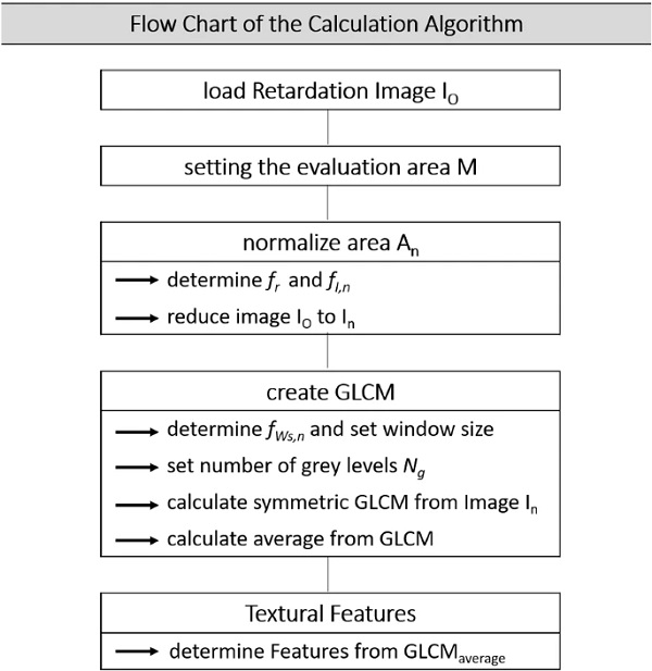
The flow chart in Fig. 10 represents a scheme by which textural features can be extracted step by step from the original retardation image, independent of the glass format. The normalization of the reference area, the calculation of the geometry factors, the formation of the GLCM and the determination of the textural features is accomplished in a calculation algorithm written in the program MATLAB®.
Influence of the image size
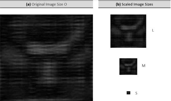
It is known from Hidalgo and Elstner (2018) that the formation of GLCM from retardation images is very computationally intensive and therefore time-consuming. The reason for this is the complex process of forming GLCM and the fact that the original retardation images have a very high resolution and therefore very large m × n matrices. One approach to reduce the calculation time is to reduce the size of the original images for the calculation of the GLCM and the textural features. The impact of this approach is examined below.
In order to ensure comparability of the results of the different glass formats (A and B), the original retardation images from Sect. 2.3 were scaled to fixed sizes as proposed in Sect. 4.2.1. The scaling was achieved by the algorithm of "nearest-neighbor interpolation" and was classified into the three image sizes small S, medium M and large L from Table 3. The effects of image size reduction on the textural features Contrast (C) and Cluster Prominence (CP), the global criteria x95, Iso75 and the calculation time were investigated. In this analysis, the calculation time (CT) includes the time required to form the individual GLCM. These were calculated with the step size dS = 13 px, dM = 67 px and dL = 135 px for format A, which corresponds to approximately 100 mm.
As number of the grey levels Ng=256 was chosen. The image processing algorithms were applied with the program MATLAB® on a mid-class PC without parallelization of the CPU or use of the GPU. A remarkable deviation between the global characteristics xL,0.95, xM,0.95 and xS,0.95 as well as IsoL,75, IsoM,75 and IsoS,75 could not be identified. The results of the texture features CL, CM, CS and CPL, CPM, CPS differed only insignificantly between the image sizes original to small. In return, the computation time of the GLCM is considerably reduced.
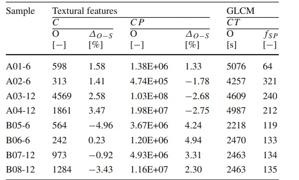
As an example, in Fig. 11 the results of the texture feature C and the calculation time of the GLCM (CT) for the sample A-01-CF-TSG-6 are compared. Table 4 shows a simple percentage deviation ΔO−S of less than 5% between the results of the feature C and CP of image sizes O and S. However, the calculation time (CT) of the GLCM was reduced from more than 5 s for the original image size O to less than 0.08 s for the format size S. For all investigated samples this corresponds to an average speed-up factor fSP of 170, which is the quotient of CTO and CTS.
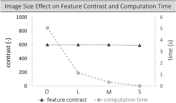
Table 4 Influence of reduced image size of features C, CP and CTGLCM - Full size table
The study has shown that with the same ratio of step size to image size, the textural features C and CP have changed only irrelevant. The use of reduced images while keeping to the geometry factors can therefore be recommended to evaluate different sample geometries.
Influence from GLCM settings
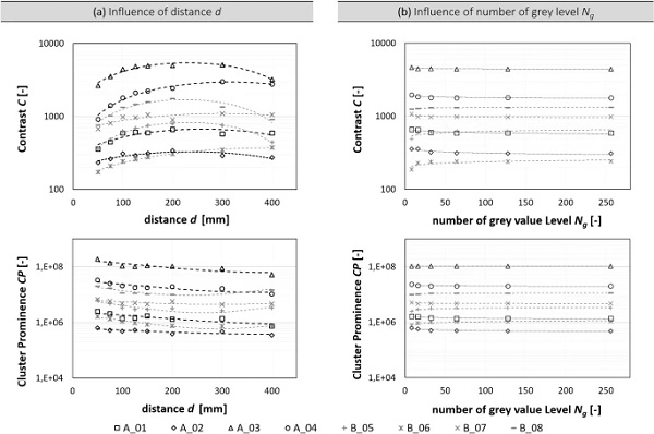
Since there is insufficient experience in applying texture analysis to retardation images resulting from inhomogeneities in the production of thermally toughened glass, a series of parameter studies will be conducted to evaluate the effects of the parameter step size and number of grey value level (Ng) of the GLCM on the results of texture analysis. Therefore, based on the experience of the previous studies, different distances d from 50 to 400 mm are applied to retardation images of reduced size S.
In Fig. 12a the results of the feature C and CP are shown as a function of the distance d. These results show that there is a significantly change with the variation of d. At the beginning it appears that with increasing d the contrast value also increases. However, this statement can only be made individually for step sizes smaller than 200 mm. In addition, the results show that the values at a distance of 400 mm should not be trusted when applied to retardation images with a width of 720 mm. This statement is also transferable to the results of the textural feature CP. Therefore, it is necessary to define a standardized step size for the formation of GLCMs. A recommended distance of 100 mm can be given based on the study.
Table 5 Comparison of the results of all calculated evaluation criteria which were applied to the retardation images from Fig. 13 - Full size table
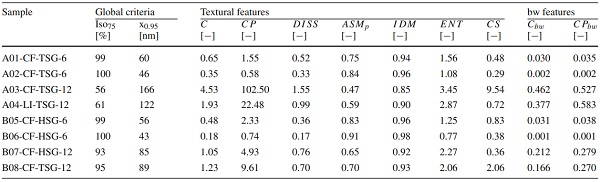
The intensities of the grey values occurring in our images have retardation values from 0 to 255 nm. Therefore, the number of grey levels was previously set to 256 when the GLCM was formed. In the following we will investigate how number of grey levels affect the results of the textural features C and CP, as well as the calculation time. For this purpose, retardation images with the reduced size S were used and the GLCMs were formed with a step size of 100 mm. In the study the GLCM parameter Ng is varied in steps of s=8,16,32,64,128 and 256.
In the calculation algorithm of the function "graycomatrix" in Matlab®, this is generated by scaling the retardation values in the greyscale image to integers between 1 and the selected level s. From the newly scaled image the GLCM is then formed and the textural features are determined. The previous very abstract values of the Table 4 are transformed into more simple values in Table 5. Comparing the two tables and considering e.g. the feature CP of sample A01, the values change from 1.38E + 06 at Ng=256 to 1.55 at Ng=8.
In order to show how the influence of different Ng affects the results of the textural features, these are normalized after the calculation. Using the knowledge of the nonlinear relationship of Eqs. (7 and 8), the normalization can be determined and mathematically expressed as:
Figure 12b shows the results of this examination for the feature C and CP. If no significant deviation from Ng=256 is recognizable between Ng=128 and 16, there is a slightly deviation of the results at Ng=8. However, the basic statement of the textural features does not change. The calculation time of the GLCM is reduced by about half from t256 to t8. Compared to Sect. 4.2.2 this is only marginal, but worth mentioning.
Threshold and texture analysis
The simplest greyscale image is an image with only two intensities: Black and White. In this investigation the combination of threshold and texture analysis will be tested. Therefore the simple global threshold from Sect. 3.2 with a limit value of 75 nm generates exactly these binary images from the retardation images, see Fig. 6a. By using T75 a new pattern is created in Fig. 6b. A GLCM with a number of grey level Ng = 2 is then formed on this BW image as before and the textural features Cbw and CPbw are determined.
The results of this study with application on all glass samples from Sect. 2.3 are shown in Table 5 under the heading of bwfeatures. It can be seen that for samples with Iso75 values close to 100% no textural statement is possible, since few or no values are available for an analysis. For samples with high x0.95 values (e.g. A03) very high retardation values are not considered as such. Since by setting the threshold of T75 the texture analysis cannot distinguish between values of 77 nm and 220 nm. The evaluation of the results of the features Cbw and features CPbw should therefore be treated with caution. When evaluating the calculation time, it is noticeable that it is not reduced. The application of the combination of threshold and texture analysis is therefore only possible to a limited extent and requires further research in the future.
Evaluation further textural features
The feature C and CP have already proven their suitability in Hidalgo and Elstner (2018). In this section we will check if the calculation of further textural features from section 3.3 (Eqs. 11, 12, 13, 14, 15) are also useful for evaluating retardation images. In principle, a feature is sought that can detect and evaluate the inhomogeneity of the images, i.e. the frequency of an intensity change and contiguous areas with high intensities. For this study, symmetrical averaged GLCMs of the retardation images were formed using the procedure from Fig. 10 with d = 100 mm and Ng = 8. The results of the further textural features are shown in Table 5.
The similarity of the features C and DISS in their formulas, see Eqs. (7) and (11), is also reflected in their results. Due to the equality to C, one of the two features is probably obsolete for further investigations. Based on the positive experience with C this is further used. The results of the features Angular Second Moment (ASM) and Entropy (ENT) also determine the texture homogeneity of the images very well. Thus, with ASM = 0.91 and ENT = 0.77 they detect a homogeneous retardation image for sample B06 and an inhomogeneous retardation image for sample A04 with ASM = 0.59 and ENT = 2.87.
However, no significant difference is discernible between the values of sample A04 and sample B07, although the global evaluation criteria differ significantly for these. IDM (Eq. 13) recognize inhomogeneous and homogeneous images, but the values differ only marginally from 0.85 to 0.98, so that only a tendency can be read and a further use is currently not recommended.
Feature CP captures contiguous areas of higher retardation and is therefore well suited for use in retardation images. Cluster Shade (CS) is similar to CP according to the Eq. (15). However, when comparing the results of both features, it is noticeable that the values for samples A04 and B07 do not correlate. Since the statement of CS cannot be reproduced, it is not recommended.
The investigations have shown that the further textural features DISS, ASM, IDM, ENT and CS are indicators for inhomogeneous images, but are not a superior alternative to the proven features C and CP proposed by Hidalgo and Elstner (2018).
Final evaluation of retardation images
Evaluation of the 6 mm glass panes
Finally, the retardation images from Fig. 13 can now be evaluated and compared according to the presented criteria. Since it is known from Eq. (1) and previous investigation FKG (2019) that glass thickness has an influence on the occurrence of optical anisotropies, samples with a thickness of 6 and 12 mm are considered separately in the further evaluation.
If one considers the 6 mm glass panes, it is immediately apparent that when a threshold of 75 nm is set, all four samples have an Iso 75 value greater than 99 percent. A comparison between the quality of the samples does not allow this criterion in this case. In order to obtain meaningful values for these samples, the threshold value for this glass thickness would have to be lowered to e.g. 50 nm. The evaluation according to quantiles such as x0.95 is therefore better suited to assess the glass quality. However, as in this case, an evaluation according to the exclusion zones from Sect. 4.2.1 should be performed. The statistical x0.95 values of samples A01, A02, B05 and B06 are in the range of 43–60 nm. x0.95 classifies A01 as worst of the four panes.
If the textural features C and CP are considered individually, C classifies the homogeneity of the retardation images and CP classifies coherent areas with high retardation. Sample A02 and B06 with low C and CP values are classified as higher quality glass panes. A01 with its overall inhomogeneously distributed retardation has a higher C value of 0.65 than B05 with 0.48, which implies a more frequent variation between lower and higher retardation values. Sample B05 with its punctual high retardation and slightly developed middle stripes, however, also has larger areas with only very low retardation. This results in a lower C value but a higher CP value.
A statement, which texture feature should be weighted more strongly in the evaluation, cannot be given at present. A combination of the two texture features is therefore of interest for future research.
Evaluation of the 12 mm glass panes
In the evaluation of the 12 mm glass panes, samples A03 and A04 show significantly higher retardations over the area compared to samples B07 and B08 with medium coherent retardation areas. All criteria from Table 5, classify them as worse anisotropy quality and also rate A03 as the most striking sample. In the evaluation, the Iso 75 values vary in the range from 95 to 56 percent and the x0.95 values from 85 to 166 nm. The texture analysis provided more detailed differentiation between samples B07 and B08, which were both classified as good. It is obvious that although the retardation images differ in the spatial arrangement of the intensities, the results of the global evaluation criteria hardly change. C and CP weighted the stripe pattern with high retardation from B08 as more striking and therefore worse than sample B07. Nevertheless, these glass panes could be classified as good quality and should cause less anisotropy when installed in the façade.
Conclusion and future research
In the presented paper optical anisotropy effects in thermally toughened architectural glass are quantified by full-field photoelastic measurements and evaluated by different methods of digital image processing. When applying global methods on the acquired retardation images, it was shown that statistical methods, such as the x0.95 quantile value, are in principle preferable to threshold methods for the comparison of different anisotropy qualities, since these depend strongly on the choice of the threshold T. The introduction of evaluation zones according to Bundesverband Flachglas (2009) avoids a falsification of the statistical characteristic values caused by high retardation values near the edge area of the glass panes.
It was shown that the resulting anisotropy patterns of the tempered glass panes investigated in this study can be further evaluated with texture analysis based on the Grey Level-Co-occurrence Matrix. The main advantage of texture analysis compared to statistical or threshold methods is the integration of the spatial arrangement of retardation values into the evaluation. A method was proposed which permits comparable results despite different glass formats and achieves an enormous speed-up in the calculation time of the GLCM. In addition, it was demonstrated that the choice of the setting parameters of the Grey Level Co-occurrence Matrix has a decisive influence on the results of the textural features and therefore has to be determined as proposed in this paper.
The novel method with calculation of the textural features Contrast and Cluster Prominence can now be implemented e.g. together with statistical parameters in online measurement systems. In this way, the anisotropy quality of the glass pane can be evaluated and optimized in the production process so that the disturbing visibility of anisotropy effects in façades is reduced in the future. In further investigations retardation measurements have to be performed on a variety of different thermally toughened glass panes. On the basis of these investigations, the evaluation criteria can then be proven and quality standards defined.
Acknowledgements
The authors would like to thank the Fachverband Konstruktiver Glasbau e.V. for their support, especially the members of the working group "Anisotropy", who made it possible to realize these investigations by providing the test samples.
Funding
Open Access funding enabled and organized by Projekt DEAL.
Author information
Authors and Affiliations
Institute for Material and Building Research, University of Applied Sciences, Munich, Germany
S. Dix, P. Müller & C. Schuler
Institute of Mechanics and Materials, THM University of Applied Sciences, Giessen, Germany
S. Kolling
Institute of Structural Mechanics and Design, Technical University of Darmstadt, Darmstadt, Germany
J. Schneider
Corresponding author
Correspondence to S. Dix.