This paper was first presented at GPD 2023.
Link to the full GPD 2023 conference book: https://www.gpd.fi/GPD2023_proceedings_book/

Authors:
- Lorenzo Santi - University of Parma, Italy
- Stephen Bennison - Kuraray America Inc, Wilmington DE, USA
- Michael Haerth - Kuraray Europe GmbH, Troisdorf, Germany
- Gianni Royer-Carfagni - University of Parma, Italy
Abstract
We discuss an innovative approach, also mentioned in next-generation Standards, which uses the mathematical tool of fractional calculus to interpret the interlayer viscoelastic properties of laminated glass. Reference is made to the paradigmatic example of a simply supported laminated glass beam under longduration loads. The comparison with the more traditional approach based on the Wiechert model, and the consequent approximation via Prony series of the relaxation function of the polymer, indicates two main advantages: the definition of the model parameters from experimental data is greatly simplified; the numerical implementation is easier and computationally more efficient.
Introduction
It is well-known that the capacity of laminated glass in the pre-breakage phase depends upon the shear coupling of the glass plies through the polymeric interlayers. Although the interlayer is viscoelastic, most design calculations follow the quasi-elastic approximations, in which the polymeric film is considered linear elastic, with an effective shear modulus calibrated on the duration of applied actions and operating temperature. This is certainly a consolidated approach, reported in Standards [1], which can be used in most conditions. However, when impulsive actions are applied (impact, blast waves), and even more so when the load is not monotone, the hereditary memory of viscoelasticity, neglected in the quasi-elastic approximation, may play a significant role. In such cases, a full viscoelastic analysis is required.
The rheological properties of laminated glass are dictated by the viscoelastic properties of the polymeric interlayer. The theoretical modelling relies on Boltzmann’s superposition principle and requires, as input datum, the relaxation function of the polymer, indicating the decay in time of the secant elastic modulus in a homogeneously strained specimen.
Experiments on most commercial polymers [2] indicate that the relaxation function can be well approximated by branches of power laws of time. In a bi-logarithmic plot, these correspond to a polyline, each segment of which is completely described by two parameters, i.e., its slope and the intercept with a vertical axis. In general, as it will be shown later on, three segments are sufficient to characterize the long-term response in most cases; hence, six parameters are sufficient for an exhaustive description, whose calibration presents no difficulty because of the intuitive geometric interpretation. On the other hand, the traditional approach based on the classical Wiechert model, requires an approximation of the relaxation function in Prony series of exponential functions of time, each one characterized by a characteristic relaxation time. To obtain reliable results in a wide period of observation, at least 20-30 parameters are needed, whose calibration from experimental results is not straightforward [3].
There is a mathematical description of the equations of viscoelasticity, founded on fractional calculus [4], which naturally provides power laws of time as fundamental solutions. The scope of this work is to demonstrate, in paradigmatic examples, the great advantages of the fractional viscoelastic approach over the traditional characterization via Prony series. Therefore, it is not surprising that this innovative approach has been mentioned in the background documents of the new CEN/TS 19100 – Design of glass structures [1].
The model
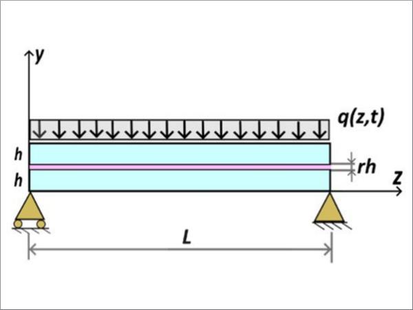
Consider, as an illustrative example, a simply supported three-layer beam, composed of two glass plies of thickness h, coupled by a thin polymeric interlayer of thickness s = r h, with r<<1. The beam has length L and width b; the cross-sectional area of each ply, considered as a Euler-Bernoulli beam, is A = b h and the moment of inertia of each ply, is I = bh³/12.
The total beam mass per unit length is μ [Kg/m] and it is calculated by multiplying the glass density [2500 Kg/m³] by the cross-sectional area (the interlayer mass is neglected). The beam is subjected to a distributed load per unit length denoted with q(z, t), as indicated in Figure 1.
The interlayer, shear-coupling the glass plies, is supposed to be so thin that shear stress is homogenous through its thickness, which remains unaltered under the applied load. The equilibrium equations for the fractional viscoelastic model and the Prony series approach can be found in [5] for the case of bomb blast loading, characterized by a time scale so small that the relaxation function can be described by only one branch of power-law (one straight line in the bi-log plot) in the significant interval of observation. Now, the description is extended to longer times, so that more branches of power law are required.
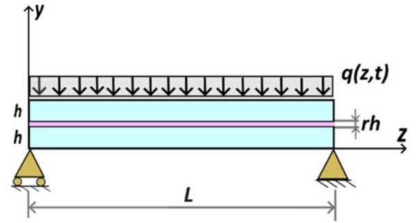
Suppose, for simplicity, that the applied load is uniformly distributed, but it varies in time as shown in Figure 2. The load starts from zero and it linearly increases, reaching the plateau q = 3 kPa in approximately 1 hour. This value is representative of the pressure on floors in public areas (category B/C1) according to EN 1991-1-1.
Characterization of material properties
The viscoelastic characterization of the polymeric interlayer is now illustrated by comparing the fractional calculus and the Prony series approaches. The most natural way to approximate the relaxation function in the fractional approach is a power law, or continuously connected branches of power laws, of the type R(t)= Cₙ t ⁽⁻ⁿ⁾, with 0 < n < 1, where R(t) is the time-dependent secant shear modulus, with the time t usually expressed in seconds. In a bi-log plot, a power law appears as a straight line. For a commercial polymer, in a longer time scale of observation, the relaxation function is typically of the shape represented in Figure 3, such that it can be conveniently approximated by using three branches of power laws, corresponding to a trilateral in the bi-log plane. Each segment is defined by 2 parameters: Cₙ, representing the “stiffness” of the viscoelastic material (value at t =1 s), and n, which is the slope of the line. For shorter intervals of observation, it could be sufficient to consider only two branches or just one power law.
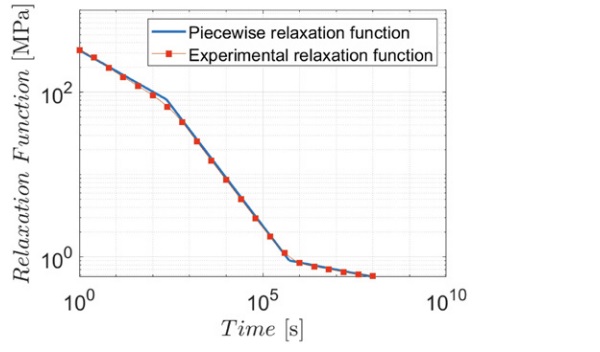
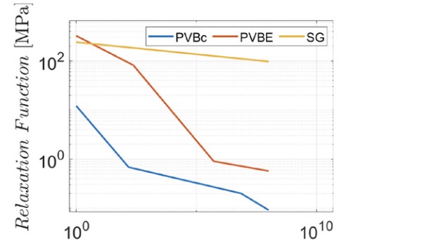
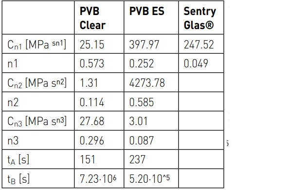
Figure 4 shows the relaxation functions for three different interlayer materials, all produced by Kuraray Europe GmbH, i.e., PVB Clear, PVB ES and SentryGlas®, approximated with branches of power laws. The experimental data have been provided by Centelles et al. [6], who conducted creep test for a period of four months on laminated glass panes under uniformly distributed load. Observe that, to describe the SentryGlas® interlayer, only one power law is sufficient also for such a long observation time; on the other hand, three branches are needed for PVB Clear and PVB ES. The parameters used to approximate the relaxation function with power laws have been calculated in [7] and are now reported in Table 1.
The numerical implementation of the fractional viscoelastic model requires the recursive construction of a triangular matrix, which can be readily calculated from such parameters following the procedure described in [7]. This matrix is at the base of the Grünwald-Letnikov method to solve the system of fractional differential equations. The problem is solved à la Galerkin, as in [5], by considering an expansion in Fourier series of the beam deflection: in general, only three terms of the series are sufficient to achieve a reliable approximation.
Alternatively, the relaxation function can be described via Prony series of exponential functions, which interpret the Wiechert model consisting of an array of Maxwell units in parallel with a spring of stiffness R₀, which represents the stiffness of the viscoelastic material when time tends to infinity. Each term of the Prony series is of the form Rᵢ e⁽⁻ᵗ⁄ᶿⁱ⁾), where Rᵢ is the i-th relaxation shear modulus and ϑᵢ its corresponding relaxation time, such that R(t) = R₀ + Σⁿ (Rᵢ e⁽⁻ᵗ⁄ϑⁱ⁾). Figure 5 represents the relaxation function of PVB Clear and its approximation using six (i = 6) terms of the Prony series, corresponding to 13 parameters to be calibrated. Observe the “wavy” character of the resulting curve.
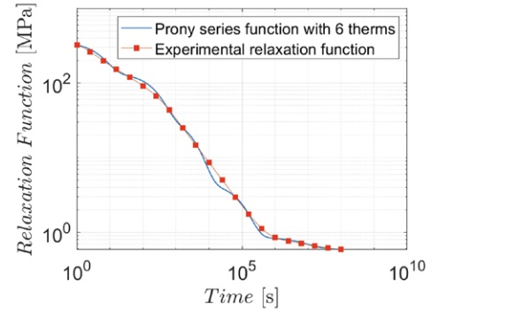
The fractional viscoelastic approach has two main advantages over the Prony series approach. The first is that material characterization is simplified. Indeed, to represent the relaxation function with the fractional model, six parameters are needed for a trilateral function (only two parameters for SG); instead in the Prony series, at least thirteen parameters are needed as shown in Figure 5, but if a higher accuracy is required (“less wavy” curve) a larger number of terms is necessary.
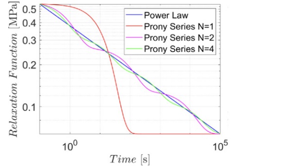
Figure 6 demonstrates how the accuracy of the relaxation function increases by increasing the number of Prony terms. Indeed, each term of the Prony series is associated with a sudden stiffness decay at the characteristic time ϑᵢ , so that the relaxation function results from a sequence of “falls”. Whereas the experimental data are well approximated by segments in the bi-log plot, the problem is now to interpolate a line with a sequence sigmoid-like curve.
Numerical analysis
The benchmark problem for the simply supported laminated glass beam has been solved for PVB Clear and PVB ES interlayers. The deformation of the beam is interpreted by the maximum vertical displacement v(z/2 ,t) at midspan. The geometry is provided by the length L = 1.5 m, width b = 1 m and height h = 8 mm. The polymeric interlayer has thickness s = rh = 1.52 mm (with r = 0.19). The Young’s modulus of glass is set equal to E = 72 GPa.
The solution of the fractional viscoelastic problem has been obtained using the Grünwald-Letnikov integration scheme [7]. For the Prony series, the traditional approach is the finite difference method [7]. The coefficient of the series has been obtained with the “Domain of influence method” [3], which represents a practical approach to calculate R₀, Ri and ϑᵢ starting from the experimentally measured relaxation function.
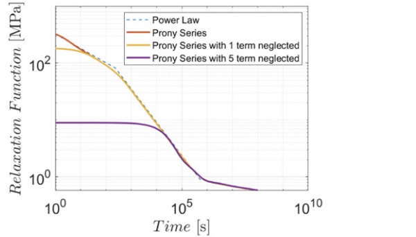
It is necessary to mention a difficulty that it is generally encountered when solving the differential system of equations via the finite difference method. The terms of the Prony series that correspond to a relaxation time ϑᵢ smaller than the integration time step Δt (obtained by dividing the total observation time in several equal intervals) can in general cause numerical problems, because of the poor approximation of the time derivative with the incremental rate of change. A practical way to bypass this problem is to neglect the terms with ϑᵢ << Δt in the series. However, this implies an overestimation of the maximum deflection because the relaxation function becomes flatter and assumes lower values for small time scale, as shown in Figure 7.
If our goal is to analyse the response of the beam for small time scales, this simplification is not necessary because all the relaxation times ϑᵢ are higher that the step time Δt. However, to follow a long-term phenomenon, the time step shall be conveniently increased, otherwise the number of steps would become excessively large.
Numerical integration for both the Prony series and the fractional approach has been implemented in MATLAB. The displacement at the beam midspan has been calculated for two different periods of observations: three hours, to estimate the effect of the loading phase; four months, for the long-term creep. The two materials (PVB ES and PVB Clear) characterized by a trilateral relaxation law in the bi-log plane, have been compared.
Important reference values are the deflections at the layered and monolithic limits. These are calculated as 5/384·(qL⁴/EI) by setting either I = 2(bh³/12) or I = 2(bh³/12) + (1+r)²h²A/2 for the layered and monolithic cases, respectively. This calculation provides 32 mm and 6.1 mm.
Figures 8 and 9 shown the displacement as a function of time for PVB ES and PVB Clear, respectively. During the loading phase (Figures 8a and 9a), corresponding to a period of observation of the order of 10⁴ s, 2000 time-steps have been used, corresponding to Δt = 5 s for both the fractional and the Prony series approach.
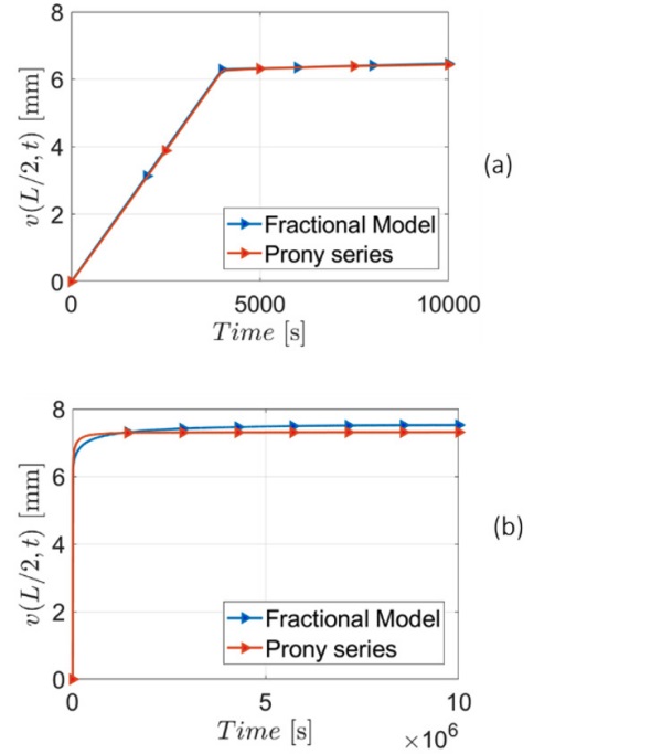
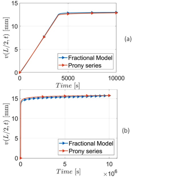
In the Prony series only the first term has been neglected because the relaxation time was lower that the step time (ϑᵢ < Δt). The relaxation function corresponding to PVB ES is therefore the yellow curve of Figure 7. The accordance with the solution of the fractional model is very good: the difference is 0.4% for PVB ES and 0.87% for PVB Clear.
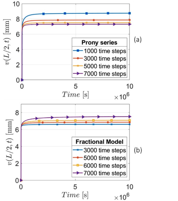
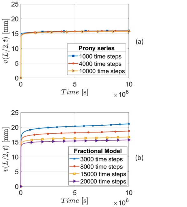
Figures 8b and 9b correspond to the long creep, i.e., a period of the order of 10⁷ s (~4 months). For the Prony series solution 7000 time-steps have been chosen for PVB ES (Δt =1.4·10³ s) and 10000 time-steps for PVB Clear (Δt = 10³ s). In both analyses, the first five terms of the Prony series were neglected because their relaxation times were lower than the time step. The corresponding relaxation function PVB ES is the violet curve in Figure 7. Observe that the number of time steps required to achieve convergence is different for the two materials used as interlayer. Figure 4 clearly indicates that PVB ES interlayer is stiffer than the PVB Clear; the results for PVB ES are in fact closer to the monolithic limit.
Convergence Analysis
The advantages of the fractional viscoelastic model over the Prony series approach become more evident in terms of computational performance. Figures 10 and 11 illustrate the results for the long-creep solution, respectively for PVB ES and PVB Clear, in their comparison between the fractional and the Prony series approaches. Both solutions have been obtained by implementing in MATLAB the numerical method (finite difference for Prony series; Grünwald-Letnikov for fractional viscoelasticity). The analysis of the first loading phase presents the same qualitative characteristics as the long-creep phase and it is not reported for brevity.
The convergence analysis consists in calculating the solution by varying the integration time step.
The solution reaches convergence when it does not considerably vary by further decreasing the time step.
In the case of PVB ES interlayer, both the Prony series and the fractional approaches converge to the same curve, but the required number of time steps is different. Observe that in the Prony (fractional) approach the solution is approached from above (below). The PVB Clear case is characterized by a faster convergence of the Prony series approach. The solution for the fractional model is now reached from above. The different trend observed for the two materials is dictated by the shape of their relaxation functions, represented in Figure 4.
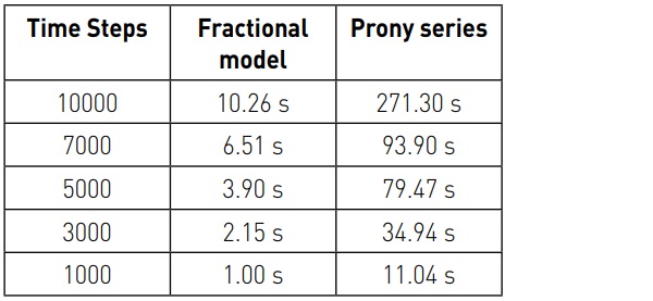
However, results should be compared in terms of computational cost. Table 2 records the time required to calculate the numerical solution with the fractional and the Prony series approaches. It is evident from the data that the fractional model is computationally much lighter than the Prony series approach. A reason for this is that in the GrünwaldLeitnikov mathematical formulation it is not necessary to calculate the relaxation function at each time step, as in the finite difference method used for Prony series, since the solution relies on schemes that requires the inversion of the triangular matrix. Enlarging the time-step, a few terms of the Prony series had to be neglected to avoid numerical errors: although some precision is lost, the computational time diminishes, but in all cases the fractional approach remains computationally convenient.
Conclusions
Two mathematical approaches have been compared, applicable in the modelling of the viscoelastic behaviour of polymeric interlayers, which determine the rheological response of laminated glass under applied actions. The first is the classical one, based on the approximation of the relaxation function of the interlayer in Prony exponential series; the second one makes use of fractional calculus for the definition of Boltzmann's superposition principle, at the basis of the theory of viscoelasticity. The latter formulation provides, as direct solutions, functions described by power laws over time.
Starting from the experimental observation that in most commercial polymers the relaxation function can be piecewise described by power laws, the fractional approach appears particularly suitable for modelling laminated glass. The numerical implementation through the Grünwald-Letnikov method does not present difficulties. The convergence analysis has shown noteworthy advantages over the solution via the finite difference method of the classical differential equations, based on the Prony series expansion.
This study confirms why the approach based on fractional calculus for the viscoelastic analysis of laminated glass should be seriously considered for incorporation in next-generation standards.
References
[1] Feldmann M., et al, The new CEN/TS 19100: Design of glass structures, Glass Struct. Eng., Published on line 2023, doi.org/10.1007/s40940-023-00219-y.
[2] Biolzi L., Cattaneo S., Orlando M., Piscitelli L., Spinelli P., Constitutive relationships of different interlayer materials for laminated glass, Composite Structures, 244, 112221, 2020.
[3] Gant F. S, Bower M. V, Domain of influence method: a new method for approximating Prony series coefficients and exponents for viscoelastic materials, J. Polym, 17 (1), pp. 1–22, 1997.
[4] Tarasov V. E., Leibniz rule and fractional derivatives of power functions, Journal of Computational and Nonlinear Dynamics, 11(3), 031014, 2016.
[5] Viviani L., Di Paola M., Royer-Carfagni G, Fractional viscoelastic modelling of laminated glass beams in the pre-crack state under explosive loads, Int J Solids Struct, 248, 111617, 2022.
[6] Centelles F., Pelayo A., Lopez M., Castro J. R., and Cabeza L. F., Long-term loading and recovery of a laminated glass slab with three different interlayers, Constr Build Mater., 287, 122991, 2021.
[7] Viviani L., Di Paola M., Royer Carfagni G., Piecewise power law approximation of the interlayer relaxation curve in the long-term fractional viscoelastic modelling of laminated glass, Submitted, 2023.