Authors: Alexander Pauli & Geralt Siebert
Source: Glass Structures and Engineering 9(1):1-15
DOI: 10.1007/s40940-023-00236-x
Abstract
Recently, the numerical simulation of the residual load-bearing capacity of laminated glass (LG) is an often discussed but not sufficiently solved problem in structural glass design yet. According to CEN/TS 19100:2021 (2021a), and CEN/TS 19100:2021 (2021b), the design in the Post Fracture Limit State (PFLS) is possible experimentally and numerically. Experimental verification requires large-scale component tests, which are often costly and time-consuming. The resource-saving numerical approach is to be preferred. However, at the moment, there is no sound numerical model capable of representing the complex load-bearing mechanisms of broken laminated glass (LG) in civil engineering practice. These mechanisms are the finite-strain response of the interlayer, the contact between glass fragments or shards themselves, and the bond between glass and interlayer. Delamination governs the latter one mainly. This work focuses on the experimental, mechanical, and numerical characterization of the finite-strain behavior of polymeric laminated glass interlayers at long load durations by the example of standard single-layer Polyvinylbutyral (PVB). Based on that, it introduces an approach enabling the simplified numerical simulation of LSG interlayers. The considerations rely on experiments and thermodynamic considerations.
1 Introduction
Nowadays, glass is one of the most popular building materials, especially in light transparent structures. According to the “fail-safe approach” in structural glass design (Feldmann et al. 2014), the glass structure must provide sufficient stiffness and strength in the case of partial or total fragmentation. Monolithic glass suffers from brittle failure and shows no residual load-bearing capacity. Therefore, laminated glass (LG), or rather laminated safety glass (LSG), must be used to meet this requirement. To quantify or prove the residual load-bearing ability of laminated glass, the standards require carrying out component tests. However, these investigations are very time- and cost-consuming. A different way of quantifying the residual load-bearing capacity is the numerical investigation. Two possibilities exist for this approach: (1) an explicitly formulated model that considers all components and load-bearing mechanisms; (2) a homogenized model that considers one effective stiffness for the broken laminate. Depending on the support conditions, a failure criterion must be chosen for both cases. It could be a maximum deflection of the glazing or a specific maximum strain derived from the pure interlayer. However, determining a failure criterion is not part of this work. The paper focuses on the characterization of the interlayer in the context of residual load-bearing capacity using an explicitly formulated model. This model considers the following three shares: the interlayer, the friction of the glass fragments, and the coupling between the glass and interlayer.
The main structure of this paper is as follows: (1) The structure of the paper is settled, and the general problem of residual load-bearing capacity of laminated glass is explained. A brief literature review on this topic is given; (2) The general material behavior of PVB is characterized, and a framework to describe its mechanical behavior, based on rheological considerations, is provided. In addition, specimens, test setup, and testing procedure are introduced; (3) experimental results are presented and evaluated. Furthermore, material parameters are derived, and a numerical simulation of PVB at finite strains is carried out; (4) test procedure and evaluation algorithm are discussed concerning the residual load-bearing capacity of laminated glass. (5) The work is summarized, and further research is pointed out.
There are two possible approaches to dealing with the residual load-bearing capacity of fully broken laminated glass elements-the experimental and the theoretical approach. The theoretical approach is divided into numerical and analytical ones. However, theoretically describing laminated glass in the fully fractured state, it is crucial to calibrate several material parameters through experiments. Moreover, to validate the models, respective validation tests must be carried out. Therefore, a clear separation between experimental and theoretical approaches is not possible. The following section gives a quick literature review of the previous work on that topic in civil engineering. The first part of the section summarizes the experimental investigations and the analytical models aiming to describe the residual load-bearing capacity. The second part presents general numerical approaches with a focus on quasistatic loads. In the end, a summary of the investigations done on the bulk interlayer material is given. However, there is extensive research done in automotive design, as well (Du Bois et al. 2003; Timmel et al. 2007; Xu et al. 2011; Kang et al. 2015; Liu et al. 2016; Lin et al. 2018; Shahriari and Saeidi Googarchin 2020). But, as this paper focuses on civil engineering applications, only literature from that area is introduced further.
Several works experimentally investigated the overall residual load-bearing capacity of laminated safety glass for civil engineering applications. (cf.: Siebert 1999; Biolzi et al. 2010, 2016; Franz 2015; Castori and Speranzini 2017; Botz et al. 2019; Wellershoff et al. 2021; Biolzi and Simoncelli 2022).
Biolzi et al. (2010, 2016), Biolzi and Simoncelli (2022) conducted in-plane three-point bending tests until breakage on laminates made from annealed glass (ANG) and thermally toughened glass (TTG) with interlayers of PVB and Sentry-Glass (SG). Franz (2015) carried out Trough-Crack-Bending (TCB) and Trough-Crack-Tension (TCT) tests on laminates made from ANG and different interlayers. Castori and Speranzini (2017) provided out-of-plane four-point bending tests on laminates made from ANG and different interlayers. Botz et al. (2019) conducted uniaxial and Wellershoff et al. (2021) biaxial tension tests on fully fractured laminates made from TTG and PVB.
Furthermore, several approaches focus on the analytical modeling of the residual load-bearing capacity. Galuppi and Royer-Carfagni (2016) developed a model for plane-strain and plane-stress states of fully fractured laminated glass made from thermally toughened glass. This model is expanded to equi-biaxial stress-states by Galuppi and Royer-Carfagni (2017) and in-plane and out-of-plane bending by Galuppi and Royer-Carfagni (2018). D’Ambrosio et al. (2019) presents a different approach based on these models. All analytical approaches consider linear elastic material behavior for the interlayer.
There are two different modeling approaches that cover the residual load-bearing behavior under quasistatic loading from a numerical point of view: A homogeneous approach, in which all components and mechanisms together are considered as one homogenized material (Botz et al. 2019; Pauli et al. 2021), and an explicit approach, in which each mechanism is considered separately (explicitly) (Baraldi et al. 2016; Wang et al. 2018, 2021). Botz et al. (2019) provide a homogenized material on a trilinear elastic modulus for PVB, Pauli et al. (2021) provide a homogenized material on a bilinear elastic modulus for EVA, both for laminates made from TTG. Baraldi et al. (2016) introduces an approach for laminates made from TTG based on the Discrete-Element-Method (DEM), where they describe the interlayer by an elastoplastic material model and treat the glass fragments individually, connected by contact forces. However, they don’t consider friction between the glass fragments. Wang et al. (2018) use a combination of the Finite Element Method (FEM) and DEM. They divide the model into two subdomains after reaching a yield criterion representing the brittle failure of the glass. The first subdomain is presented by FEM, describing the interlayer in terms of a Mooney Rivlin material model, and the second subdomain is presented by DEM, describing the fractured glass. Wang et al. (2021) use a similar approach. However, they model the glass fragments more precisely using a combined Voronoi and FEM/DEM approach and the interlayer in terms of a plastic material model.
Furthermore, the pure interlayer has been investigated extensively over the last few years. Bennison et al. (2005), Morison et al. (2007), Iwasaki et al. (2007), Hooper et al. (2012a, 2012b), Kuntsche (2015) investigated the behavior of PVB at finite strains within the context of blast resistance of laminated glass utilizing uniaxial tension tests under very high strain rates. Elzière (2016), Kraus et al. (2017), Botz et al. (2019), Knight et al. (2022) investigated the behavior of PVB at finite strains concerning residual load-bearing capacity under quasistatic loading. Kraus and Niederwald (2017), Kraus et al. (2017, 2018), Schuster et al. (2021), Schuster (2023) explored the time-dependent behavior at small strains under the assumption of linear viscoelastic material behavior.
According to the theoretical approaches and the experimental investigations there is a gap between the actual material behavior observed through experiments and the material behavior assumed for the models. This work aims to provide a first approach to close this gap. Therefore, a method to describe the behavior of laminated glass interlayers for long-term static loads using Standard PVB is developed. It separates the time-independent part from the total material response, and describes it with a hyperelastic material. All underlaying considerations are based on sound thermomechanical assumptions.
2 Methodology
This section describes the investigated material, test setup, and the respective procedure and introduces the mechanical principles necessary to model the material behavior. It consists of the subsections: Material, Mechanical Modeling, and Test Setup and Procedure.
2.1 Material
Since PVB is the most commonly used material for LG interlayers, it is studied in this work.
Generally, PVB consists of PVB resin (75%), additives (<1%), and plasticizers (25%). The higher the proportion of plasticizer, the more the glass transition temperature is reduced. The material is created by chain polymerization of vinyl acetate, hydrolysis to polyvinyl alcohol, and acetalization with butyraldehyde. Below the glass transition temperature it shows energy-elastic material behavior, and above the glass transition temperature entropy-elastic material behavior. Furthermore, it has no crosslinks and shows amorphous thermoplastic thermo-mechanical behavior. For more detailed information about this topic, the reader is referred to Tschoegl (2012), Schwarzl (2013). In general, the material shows purely thermo-viscoelastic, isotropic material behavior. Considering isothermal, adiabatic conditions, it shows purely viscoelastic behavior (Kraus 2019; Schuster 2023).
The PVB used in this work is manufactured by the interlayer-company Kuraray and has the product-specific name Trosifol®UltraClear-B200NR. Its glass-transition temperature lies at 25°C (Kraus 2019), and its Poisson’s ratio lies around 0.47 (Kuntsche 2015). Kuntsche (2015) measured the transversal contraction of PVB at different strain rates and explored that there is no significant time-dependency. Therefore, its Poisson’s ratio can be assumed constant. However, for extremely high strain rates such as 3.5 [m/s], the Poisson’s ratio is reduced at small strains.
2.2 Mechanical modeling
From a thermomechanical point of view, the constitutive equations of a thermo-viscoelastic material model are governed by the Clausius Duhem inequality, a special form of the second law of thermodynamics (Truesdell and Toupin 1960; Truesdell and Noll 1965). It states that mechanical energy can be completely transformed to thermal energy, but not readily vice versa. Using the Helmholtz free energy (Truesdell and Noll 1965) Ψ as thermodynamic potential, the Clausius Duhem inequality in local form reads:

where:
- T equals the second Piola–Kirchhoff stress tensor (2PK)
- E equals the Green–Lagrange stretch tensor
- ρR equals the density within the reference configuration
- θ equals the temperature
- s equals the entropy
- Q equals the heat flux vector
- ∇ equals the nabla-operator.
- (˙) equals derivative w.r.t. time
For isothermal, adiabatic processes, which are considered within this work, the terms containing the change in temperature θ˙ and the heat flow Q, vanish. The reduced formulation with respect to the reference configuration reads:

This equation is the dissipation inequality and governs purely viscoelastic material behavior from a thermodynamical point of view. Viscoelasticity can be explicitly described by a time-dependent functional or implicitly by a differential equation (cf. Haupt 1993). For different strain rates, viscoelastic materials show different hystereses for the relation between stress and strain; however, the lower the strain rate, the smaller the hysteresis. For processes of velocities tending to a strain rate close to zero, the hysteresis vanishes, and only a single curve remains. This curve is referred to as the “equilibrium curve” and can be described by the theory of elasticity.
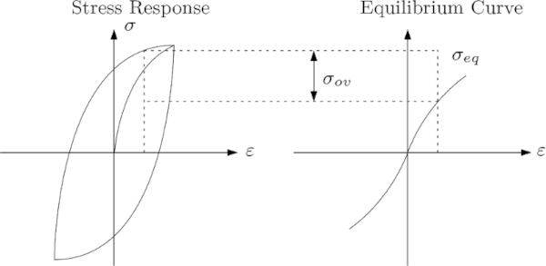
From a rheological point of view, viscoelastic material behavior can be described by the 3-parameter Maxwell model (cf. Fig. 2). Within this approach, the single spring represents the Equilibrium Curve, and the single Maxwell element represents the hysteresis. However, the spring is highly nonlinear and can be represented by a hyperelastic material.
Manipulating and solving Eq. 2, leads to the flow rule of viscoelastic material behavior at finite strains:

where Cˆel is the elastic right Cauchy–Green stretch tensor, and Dˆin is the inelastic deformation-rate tensor, both operating on the intermediate configuration. The intermediate configuration is a fictitious, stress-free state (Bergström and Boyce 1998) between reference and current configuration. The introduction of the intermediate configuration is necessary to allow the additive splitting of the deformation into elastic and inelastic parts, following the rheological approach of the 3-parameter Maxwell model, for large deformations. Lee (1969) introduced this method in the context of plasticity and Haupt and Tsakmakis (1989) expanded it to the context of viscoelasticity. Following the rheological framework of the three-parameter Maxwell model (cf. Fig. 2), the energy potential Ψ is divided into a time-dependent part Ψov and a time-independent part Ψ∞. The total stress leads to:
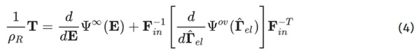
where Γˆel is the elastic stretch tensor operating on the intermediate configuration, Fin is the inelastic deformation gradient, transforming between the reference and the intermediate configuration. Considering processes at constant infinite times, the part depending on time has already been relaxed, and the resulting stress is reduced to:

From this point on Ψ∞(E)=Ψ(E) is considered for the sake of clarity. The final expression, therefore, results in:

Using , E=1/2(C-I) where C is the right Cauchy–Green stretch tensor, Eq. 6 leads to:

For the case of isotropic hyperelasticity, the material properties can be described by a single scalar function, depending on the three basic invariants (Bergström 2015) Ψ(C)=Ψ(Ic,IIc,IIIc). For the energy potential, depending on the right Cauchy–Green stretch tensor, the following relation can be derived:
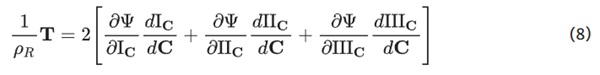
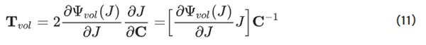
Under the assumption of isotropic material behavior, the respective energy potential can be divided into an isochoric and a volumetric part. A formulation only depending on the first invariant of the Cauchy–Green stretch tensor yields:
![]()
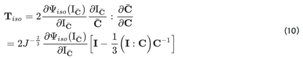
where IC¯ is the first invariant of the isochoric right Cauchy-Green stretch tensor and J the determinant of the deformation gradient F. The deviatoric part of the stress is obtained by deriving the energy potential with respect to the first invariant, making use of the projection tensor, which relates the right Cauchy-Green stretch tensor C and the isochoric right Cauchy-Green stretch tensor C¯ , resulting in

(Miehe 1994). Furthermore, the derivative of the first invariant with respect to the right Cauchy-Green stretch tensor dIC/dC = I (Chadwick 2012) is used. The isochoric part of the stress yields:
Using dIIIC/dC = IIIcC⁻¹, where IIIc = J², the volumetric part of the stress results in:
Essentially, several models are accounting for hyperelasticity. A noteworthy overview of common approaches and respective models is given by Boyce and Arruda (2000). Within this work, the potential derived by Yeoh (1990) is used for the isochoric part of the energy. It is a third-order polynomial with respect to the first invariant IC¯ of the isochoric right Cauchy– Green stretch tensor C¯ without any dependence on the second invariant. It provides greater accuracy in comparison to the Neo-Hookean potential. Compared to the Mooney-Rivlin potential, it is more stable concerning numerical stability and more efficient for computation time (Bergström 2015). Furthermore, for an uniaxial test data set, a potential based on the first invariant is sufficient. The respective potential reads:
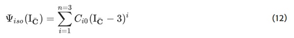
where μ = 2C₁₀ equals the initial shear modulus. However, for the volumetric part, a quite common approach is used, for instance, presented by Bergström (2015). The potential results in:

where κ equals the initial bulk modulus.
2.3 Test setup and procedure
The experimental tests were carried out in uniaxial tension mode. This assumption perfectly matches the goal of the paper, which aims to provide a straightforward repeatable concept to derive reasonable material parameters for the interlayer in the case of residual load-bearing capacity.
A single-column material testing machine from ZwickRoell (Z2.5 zwickiLine) is used. It can reach a maximum force of 2.5 kN, achieving testing velocities from 0.001 mm/min up to 1000 mm/min. A long-displacement sensor tracks and controls the deformation in the longitudinal direction at two measure points (cf. Fig. 3) using two mechanical clamps attached to the specimen. However, tests showed that the clamps do not influence the material behavior. The described device was preferred over the more common optical measurement for the following reasons. It applies the desired strain rate at the place of the measurement points and ensures a constant evaluation at the measuring points without any post-processing. Therefore, the material response at a continuous strain rate is measured directly and does not need to be approximated afterward. The experimental results are evaluated at the two measure points, and there is no need for a deformation field. The experiments were conducted in a standard laboratory climate, as it is required for residual load-bearing tests.
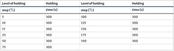
However, to ensure the repeatability of the tests, temperature, and relative humidity were continuously tracked by the temperature-humidity USB meter, Voltcraft DL-121TH. The specimen type 4 of DIN EN ISO 527-3 (2019) was used. Figure 4 shows the dimensions of the specimen. The clamps were attached in the place of the red circles. The location of these circles corresponds to the measuring length L₀ according to DIN EN ISO 527-3 (2019), which equals 50 mm. The distance between the clamps of the machine was 98 mm. The performed test is called the “staircase test” as its test procedure reminds of a staircase. This procedure is conducted to evaluate the equilibrium response of polymeric materials (Bergström and Boyce 1998). The procedure contains one cycle with a loading and unloading branch and several holding steps (cf. Fig. 5). The constant testing speed, the number of steps, the holding time, and the maximum load level is chosen individually. In this work, the strain rate is 0.01 [1/s], the number of steps is 18, the holding time is 300 s, and the maximum load level is 190% engineering strain. The unloading stops at a force of 5 N. The test procedure is presented in Fig. 5 and Table 1. For a more detailed description of the test procedure compare Table 1.
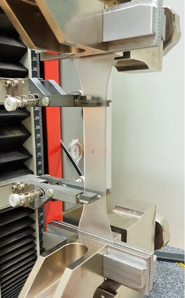
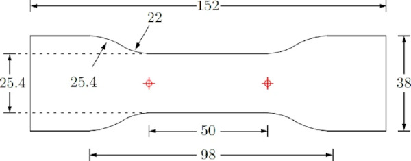
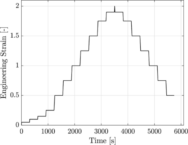
Table 1 Holding steps and times - Full size table
3 Results
This section is divided into three parts. First, the results of the experimental investigation are presented and evaluated. Second, respective material parameters for a hyperelastic Yeoh model are calibrated. Third, a numerical simulation with the commercial software Ansys is performed using these parameters.
3.1 Experimental results and evaluation
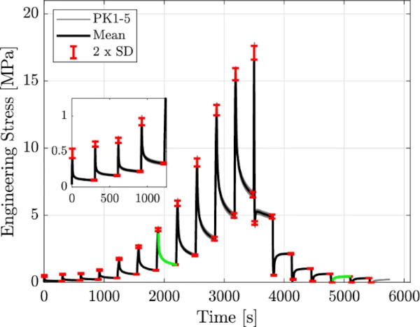
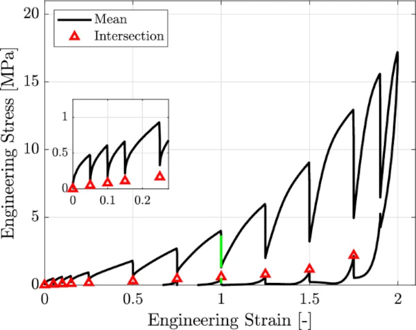
Figures 6 and 7 show the mean values of 5 tests, along with their respective standard deviations, evaluated at discrete points of the same strain value. The error bars are two times the single value of the standard deviation in length. Figure 6 shows engineering stress with respect to engineering strain, and Fig. 7 engineering stress over time.
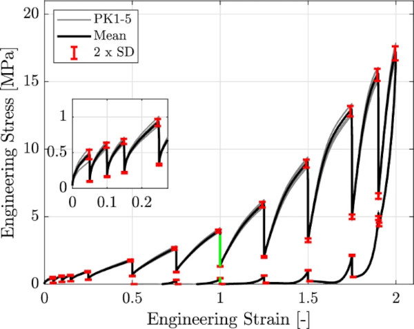
The tests were carried out at 21.5±1°C and relative humidity of 42.5±7.5% (Da Silva 2021). Temperature and relative humidity were constantly tracked (compare Sect. 2.3) but not controlled during the tests.
Figures 6 and 7 show qualitatively different material behavior on the loading and unloading branch. On the loading branch, the specimen relaxes during the holding steps, and therefore, the stress decreases. However, on the unloading branch the stress increases. This behavior can be explained by the three-parameter Maxwell model from a rheological point of view (cf. Fig. 2). On the loading branch, the spring is stretched, and a resistance force is activated. The resistance of the single Maxwell element acts in the same direction and adds up to the resistance of the single spring. The faster the loading, the more the additional resistance and the higher the tensile stress. However, if the loading is stopped and held at a constant strain level, the resistance of the Maxwell element and the overall tensile force decrease with respect to time. During unloading, the spring is released, and contracts. Now, the resistance of the Maxwell element acts against the contraction. Depending on the strain rate, this resistance force can lead to short-term compressive stresses and, depending on the geometry, to buckling.
However, if the unloading is stopped and held at a constant strain level, the resistance of the Maxwell element and the overall compressive force decreases with respect to time. The longer the strain is held, the more the compressive stress decreases and eventually becomes tensile. These considerations explain exactly the observations during the experiment. Therefore, the behavior of the holding steps on the unloading branch can be considered an actual relaxation process, and it is possible to evaluate the respective curves. Considering an infinitely slow process, the stress–strain lines run on the elastic equilibrium. Descriptively formulated, the Maxwell element drives the material away from the equilibrium curve, represented by the single spring. If the material can relax, it tends towards the equilibrium curve, which means that the stress on the loading branch must decrease and the stress on the unloading branch must increase.
Returning to the observations made during the experiments: The vertical lines in Fig. 6 show the total amount of stress in- and decrease, whereas the decaying and increasing curves in Fig. 7 show the course of the stress in- and decrease. As the steps on the loading path lay at the same strain value as on the unloading branch, it is reasonable to group each holding step at the same strain value in pairs of two (one on the loading to one on the unloading branch). For a better understanding, one representative pair of related stress in- and decrease is considered isolated in the following. This pair is marked with green in Figs. 6 and 7 at strain step 100%.
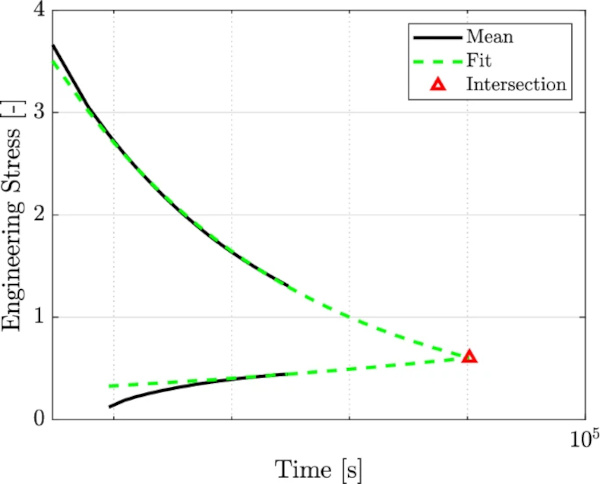
For further investigations, the stress over time behavior is examined in more detail. Therefore, the stress values of the vertical lines at strain step 100% are plotted with respect to time. For the purpose of a clearer presentation, the starting point of both lines is chosen to be at a fictitious time t = 0 s (cf. Fig. 8). Considering a double logarithmic presentation, the curve on the loading branch (upper curve) shows an almost linear course, and the curve on the unloading branch shows a nonlinear course in the beginning but tends to a linear course at a later timestep (cf. Fig. 8).
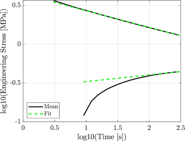
According the theory of viscoelasticity, the rate-dependent hysteresis gets smaller the lower the strain rate gets until it ends up in a single curve. Therefore, the curve on the loading and the curve on the unloading path are supposed to meet at some point in time. This point is considered to lie on the equilibrium curve, represented by the single spring of the three-parameter Maxwell model.
To find the points on the equilibrium curve, both curves (cf. Fig. 8) are fitted to a polynomial function of the first order to anticipate the courses for longer load durations. The choice of a first-order polynomial was made for two reasons. First, the relaxation curves are almost linear on a double logarithmic scale, which suggests the approximation by a first-order polynomial. Second, this ensures that the curves on the loading and unloading paths intersect. Furthermore, after the back transformation of the double logarithmic scale, a highly nonlinear curve is mapped, which represents the physical behavior of the specimen very well.
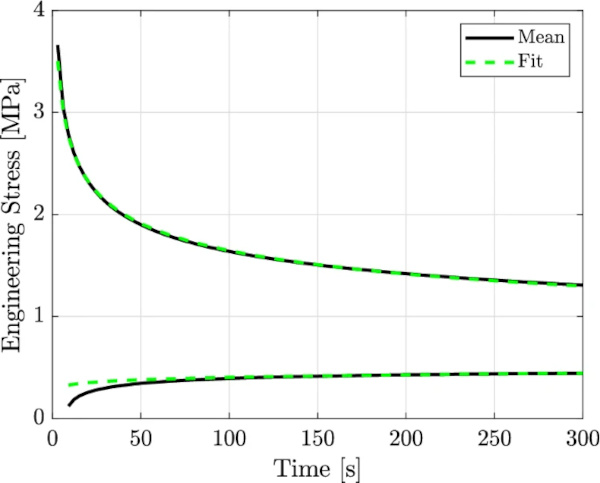
Since the behavior of the curve on the unloading branch shows only linear behavior at the end of the holding cycle, the inclination at this point is used to extrapolate the course. Figure 8 shows the curves together with their polynomial fits in a double logarithmic presentation. Having a glance at the fitted curves concerning the normal scale (Fig. 9) gives an impression of the accuracy of the fit.
Using the polynomial functions received by the fitting procedure, the intersection of the in- and decreasing stress curves can be calculated. This intersection (cf. Fig. 10) is then considered to lie on the equilibrium curve. This procedure is repeated for all pairs of in- and decreasing stress curves. Plotting the intersections within the total stress over strain curve leads to the representation of the equilibrium curve (cf. Fig. 11).
3.2 Additional remark on the experimental results
There are some things the reader should be aware of. First, the test procedure is carried out in a standard laboratory climate to represent the practical case of tests regarding the residual load-bearing capacity in the best way. The tests were carried out on different days and at various times. In the end, the mean value was evaluated.
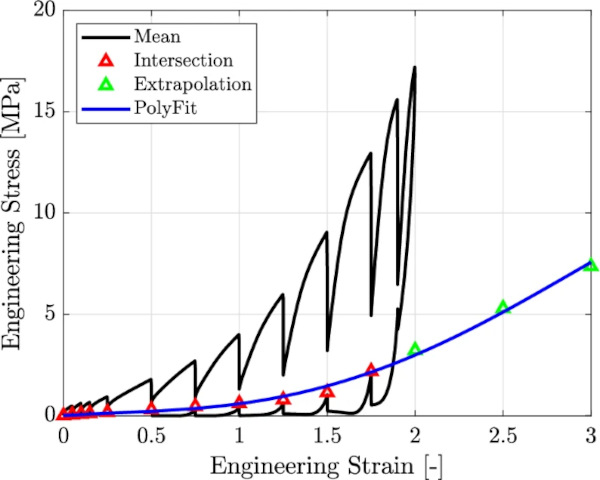
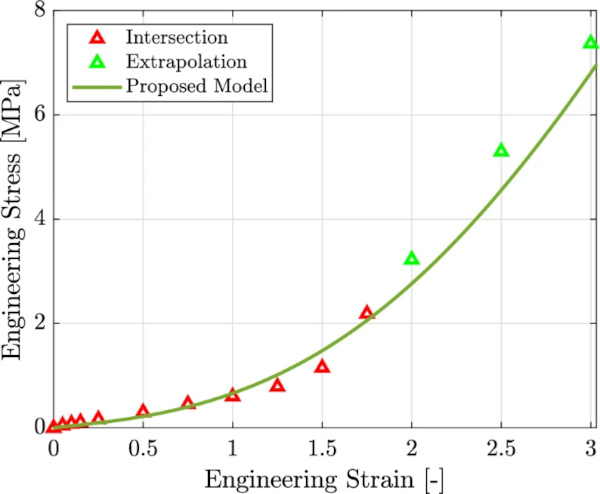
Furthermore, only pairs from 75% strain up to 175% could be evaluated using the explained procedure. For pairs below this limit, only the part on the unloading branch could be evaluated. These values are assumed to be the mean of the lowest stress of the relaxation curve and zero stress. This is only an assumption and could not be validated. The pair at strain 190% was not evaluated due to unreasonable behavior on the unloading curve. However, to provide a reliable database for the calibration of the material model, the equilibrium curve is extrapolated linearly up to 300% strain. Its inclination is calculated from the last intersection point and the one before. Subsequently, a polynomial function of the fourth order is fitted through the intersection and the extrapolated points. The derived function is then evaluated at several linearly distributed points to serve as a database for the calibration of the material model (cf. Fig. 12). The course of the evaluated points up to 175% appears to increase its inclination at every step. Therefore, the linear extrapolation is considered to be on the safe side. Figure 12 shows, that the assumption of a linear extrapolation lies on the safe side, as the curve following the points of intersection tends to harden considerably.
3.3 Parameteridentification
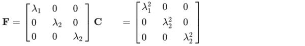
The points determined from the polynomial fit (cf. Fig. 12) serve as a database to calibrate a material model, following the theory of hyperelasticity. Therefore, the Yeoh model introduced in Sect. 2 is simplified to an uniaxial stress state to match the stress state of the experiment. λ equals the entries of the deformation gradient on the one hand and represents the stretches of the material on the other hand (λ = ε + 1). For the deformation gradient and the right Cauchy–Green stretch tensor (C = FᵀF), holds:
The engineering stress in direction of the loading yields:
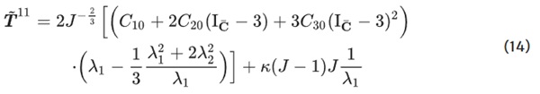
The engineering stress in transversal direction results in:
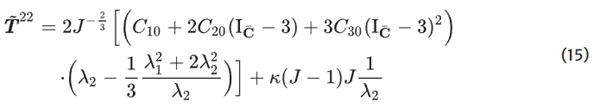
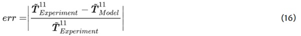
Equations 14 and 15 must be solved iteratively for the applied strain under the condition T˜²² = 0. The overall result is compared to the calibration curve, and the parameters Cᵢ₀ are derived by minimizing the error. The error is calculated by the use of the Euclidean norm (Eq. 16):
For this purpose, the “fmincon” optimization algorithm, implemented in Matlab (version R2022b), is used. That algorithm is based on an interior point technique for nonlinear programming (Byrd et al. 2000). The constraint C₁₀ > 0 is set for the optimization additionally. The chosen algorithm could already be used successfully by Kuntsche (2015), Kraus and Niederwald (2017). Furthermore, a gradient-based algorithm is a good choice concerning computation time, especially for cases where no local minima are expected.
Table 2 Parameters, adapted for FEM-model - Full size table
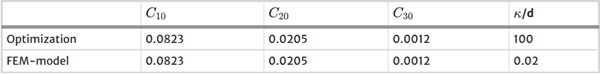
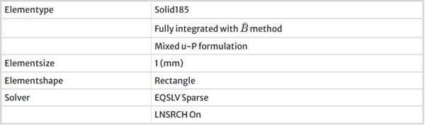
Table 3 Properties of the FEM model - Full size table
3.4 Simulation
For the simulation within this section, the commercial FEM program Ansys (version 2023 R1) (Ansys, Inc 2021) is used. The hyperelastic model based on the Yeoh energy potential Ψ = Ψiso + Ψvol implemented in Ansys is defined by:
where the initial shear modulus μ = 2C₁₀ and the initial bulk modulus equals κ = 2/d . The material parameters received from the optimization process are presented in Table 2.
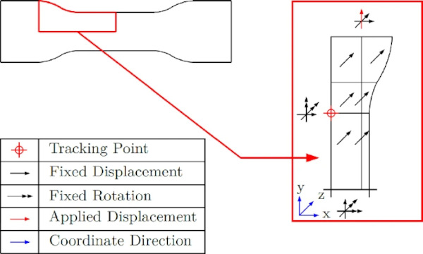
To save computation time, only a part of the specimen is modeled: a quarter in the plane and a half in the thickness direction. Figure 13 shows the respective boundary conditions that also ensure the requirements with respect to symmetry. All planes that do not move are fixed in the respective direction. Figure 14 shows the intersection points evaluated from the experiments along with the linear extrapolation and the result of the numerical simulation. The setup of the numerical model is shown in Table 3.
4 Discussion
There are numerous approaches to model the material behavior of Standard PVB in the regime of large deformations. One of the approaches, as presented by Du Bois et al. (2003), Kuntsche (2015), Kraus et al. (2017), Wang et al. (2018), is the description with a hyperelastic material model. To evaluate this approach, a distinction between short-term dynamic loads with high loading rates and long-term static loads with low rates is necessary.
For modeling the short-term, dynamic loads (cf. explosion, impacts) at very high strain rates and very short load durations, it can be reasonable to use a hyperelastic material model directly calibrated on test data (Du Bois et al. 2003; Wang et al. 2018). This approach is possible because relaxation processes do almost not affect viscoelastic materials at extremely short load durations. A reasonable approach would therefore be to fit a hyperelastic material model to data of tests carried out at very high strain rates, presented by Bennison et al. (2005), Morison et al. (2007), Iwasaki et al. (2007), Hooper et al. (2012a, 2012b), Kuntsche (2015), for instance. Following this approach in the context of residual load-bearing capacity with static loads, it seems reasonable to calibrate a hyperelastic material model on the data of a test carried out at a low strain rate or velocity (Kuntsche 2015; Kraus et al. 2017). However, this approach overestimates the stiffnes of the interlayer because its long-term behavior is governed by relaxation. Relaxation effects can not be quantified using a simple quasi-static test. That is where this work comes into play. A simple procedure to characterize and model the long-term response of PVB within the regime of large deformations is presented. Therefore, a stepwise relaxation test, referred to as the staircase test, is conducted and evaluated. The time-independent response of the material is isolated, and the viscoelastic hysteresis is reduced to an elastic curve. This curve serves to calibrate hyperelastic material models on.
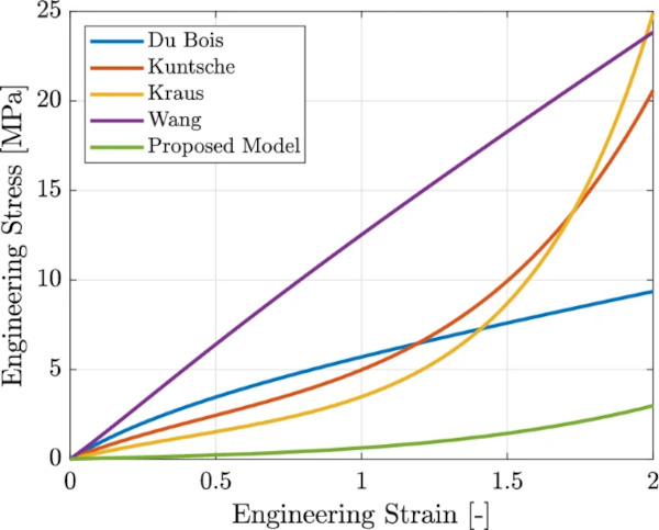
Table 4 Parameters, given from literature - Full size table
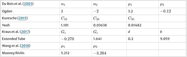
Figure 15 shows the approach of this work compared to modeling approaches found in literature (Du Bois et al. 2003; Kuntsche 2015; Kraus et al. 2017; Wang et al. 2018). Within each of these works, several hyperelastic material models are introduced. However, for the comparison in this work, only one model of each literature source is picked. Furthermore, the curves representing results from the literature were calculated analytically for the uniaxial stress state using the given parameters (cf. Table 4). All models were assumed incompressible.
Du Bois et al. (2003) used an Ogden model for crash simulations. It is calibrated on the test data provided by D’Haene (2002). Kuntsche (2015) proposed a Yeoh model, calibrated on uniaxial tensile data, evaluated at a constant true-strain rate of 0.001 (1/s). He conducted several tests at constant displacement velocities to evaluate the test data for different constant strain rates. The results of these tests are approximated by a three-dimensional surface spanned by strain, stress, and strain rate. From this surface, curves with constant strain rates can be derived. He chose the intersection along the 0.001 [1/s] strain rate to calibrate the hyperelastic material model. Kraus et al. (2017) proposed an Extended Tube model, calibrated on tension tests, carried out at a constant displacement velocity of 50 [mm/min]. Wang et al. (2018) used a Mooney-Rivlin model to simulate the impact damage of laminated safety glass. Their model was calibrated on the data of an uniaxial test at a strain rate of 125.6 [1/s]. The data was provided by Yang and Zang (2014).
The curves depicted in Fig. 15 can be assigned to three groups. The first group represents models calibrated on data of tests conducted at high strain rates (Du Bois et al. 2003; Wang et al. 2018). These results show qualitatively the same course but differ in the stress level. However, the stress level of both curves is considerably higher than the results from this work. The second group represents models calibrated on data of tests carried out at low strain rates (Kuntsche 2015; Kraus et al. 2017). The results show qualitatively the same course and also a similar stress level. Compared to the results in this work, their results show the same tendency but differ considerably in the stress level, especially at high strains. This difference becomes quite clear by having a look at Fig. 6 or respectively Fig. 7. The higher the strain, the larger the relaxation of the stress. The last group, represented by the results from this work, is based on a modeling approach without any time influences. The presented approach attempts to reduce the viscoelastic components to a minimum in order to predict the remaining stiffness after a long time duration under permanent load as well as possible.
In conclusion, the difference between the results of group one and two compared to group three lie in the difference in the approaches. Groups one and two calibrate their models on data including time-dependent, viscoelastic parts, and the approach in this work (group three) tries to avoid any influences of time.
Nevertheless, some restrictions of this approach must be pointed out. Considering thermoplastic material behavior in general, it is obvious that there is no stiffness left when time tends toward infinity. However, within the context of residual load-bearing capacity, two decisive simplifications can be taken into account. First, only quasi-static loading behavior must be considered (no cyclic loading (Elzière 2016)); second, the material behavior according to actual practice must be predicted only for 24 to 72 h. With respect to these simplified requirements, the presented method is considered to lie on the safe side. The derived material model can be used to simulate the residual load-bearing capacity of laminated glass at the end of a loading test required by the (glass) design standard.
However, to model the material behavior of laminated glass interlayers in the broken state more precisely or to calibrate cohesive zone models (Kuntsche 2015; Franz 2015; Elzière 2016), a more accurate model is required. Such a model must be able to represent nonlinear viscoelastic material behavior under large strains. It must reproduce the material response at different strain rates in the loading, unloading, and relaxation processes. One possibility would be a sum of several Maxwell elements, each with a hyperelastic spring and a nonlinear damper. The derivation of such a model is part of the current work of the authors and will be presented in future work.
5 Conclusion
A simple method to derive the finite strain behavior of Standard PVB for quasistatic loading at long load durations was presented. This method can be divided into three basic steps: first, a cyclic test with stepwise relaxation on the loading and on the unloading branch with constant holding timesteps (within the paper referred to as “staircase test”) must be carried out. Second, the relaxation steps are evaluated pairwise in a double logarithmic scale, reducing the viscoelastic hysteresis to a single curve. This curve represents the material response in thermomechanical equilibrium within the framework of viscoelasticity. Third, a hyperelastic model is reduced to a uniaxial stress state and calibrated on the curve evaluated from the experimental results. Figure 14 shows the excellent results of the numerical model.
This method showed that it is insufficient to calibrate a hyperelastic material model on the results of a quasi-static test in order to model the interlayer in the context of residual load-bearing capacity under static loads without considering the effects of time dependency.
However, the presented method is a simplified approach for modeling interlayers under long-term loading. For structural design, a failure criterion must be added. This criterion should be based on deformations. A more accurate modeling of the interlayer under different circumstances requires a model considering all time-dependent effects and influences of temperature and even humidity.