Authors: David Kinsella & Erik Serrano
Source: Glass Structures & Engineering volume 6, (2021)
DOI: https://doi.org/10.1007/s40940-021-00157-7
Abstract
Experimental strength tests are performed on two series of nominally equal plate specimens of annealed soda-lime glass subjected to either ring-on-ring or ball-on-ring bending. The Weibull effective area which represents a fictitious surface area exposed to uniform tension is calculated using closed-form solutions. Finite-size weakest-link systems are implemented numerically in a computationally intensive procedure for random sampling of plates extracted from a virtual jumbo pane whose surface area contains a set of stochastic Griffith flaws. A non-linear finite element analysis is conducted to compute the bending stresses. The glass surface condition is represented in different flaw-size concepts that depend on a truncated exponentially decaying flaw-size distribution.
Stress corrosion effects are modelled by implementation of subcritical crack growth. The effective ball contacting radius is determined in a numerical computation. The results show that surface size effects in glass are not only a matter of strength-scaling, as also the shape of the distribution changes. While the lowest strength value, as per the major in-plane principal stress at the recorded fracture origin, in the respective data sets is very similar, the strongest specimen observed in ball-on-ring testing is over 70% stronger than the correspondingly strongest specimen observed in ring-on-ring bending. The Shift function is used to make visual comparisons of the difference in quantiles in the observed data sets. Use of an ordinary Weibull distribution leads to non-conservative strength predictions on smaller effective areas, and to too low strength predictions than are viable for glass design on larger areas.
The numerical implementation of finite-size weakest-link systems can produce better predictions for the strength-scaling compared to a Weibull distribution, in particular when the flaw-size concept is modified to include a doubly stochastic flaw-size distribution or a random noise added to each subdivided region of the discretized surface area. The simulated ball-on-ring fracture origins exhibit greater spread from the centre point than otherwise observed in laboratory tests. It is indicated that the chosen representation of surface condition may not be accurate enough for the modelling of all fracture origins in the ball-on-ring setup even though acceptable results are obtained with the ring-on-ring model. There is a need for more insight into the surface condition of glass which can be conducive to the development of flaw-size based weakest-link modelling.
Introduction
Glass units are in demand in structural applications, however, the strength is challenging to predict. During its lifetime, the glass component may be subject to diverse types of loading which expose the surface area to tension zones of dissimilar size, e.g., due to uniform lateral pressure, dynamic load from a soft body impact, or a small projectile impact (Dalgliesh and Taylor 1990; Schneider and Schula 2016; Osnes et al. 2019). In addition, with modern use of glass in building construction, geometrical complexity of the glass unit can be considerable (Kozlowski et al. 2018).
A characteristic feature of glass is the dependence of strength on the size of surface area or length of edge that is exposed to tension (Vandebroek et al. 2014). However, the standard EN 16612 (2019) does not address size scaling effects. It is of great importance to be able to predict the strength of one loading configuration from the results of another. There is a need for more research on the modelling of strength and strength scaling effects in glass. The strength is defined as the major in-plane principal stress component at the fracture origin.
An experiment is carried out on annealed soda-lime glass plates of uniform dimension that are subject to biaxial loading. Two different bending configurations are used to expose the surface area to tension zones of considerably different size. The strength, fracture origin, and scaling effects are modelled in a numerical implementation of finite-size weakest-link (WL) systems using randomly generated flaws on virtual specimens. In addition, calculations of the statistical strength distribution and effective area are performed analytically using closed-form solutions for stress.
The various strength models are fitted to the laboratory data results from one of the biaxial bending setups, and then used to make predictions for the other setup, and vice versa. The results provide a basis for further discussion about the meaning and utility of the Weibull effective area in strength modelling, the relevance of taking into account fracture origins in addition to strength values when appraising the numerical models, and the potential for prediction-making of one setup based on the results from another.
Background
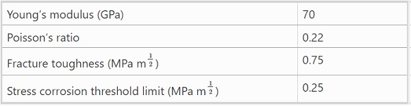
Due to the statistical nature of fracture in glass, both the magnitude of strength and failure origin exhibit random variation. The fracture origin is the source from which brittle failure begins (Quinn 2016). Fracture origins within the bulk are disregarded. The surface condition determines the magnitude of strength that is possible to attain. It is directly related to the flaws that are present and which govern the fracture phenomenon. Values for the elastic and brittle material properties are given in Table 1.
When float glass is produced, the batch is melted and floaten onto a bath of tin which produces an evenly flat surface. The side of glass that was in contact with the molten tin is called the tin-side. Annealing allows the material to cool down to room temperature while limiting the emergence of surface residual stresses. The glass is usually cut into standard size panes, socalled jumbo sheets, with dimensions 6×3.21 m² (Le Bourhis 2008; EN 572-1 2012).
Table 1 Typical values for a range of glass material properties (EN 572-1 2012; Mencik 1992) - Full size table
Previous investigations into surface size scaling effects in glass are rare, however, it was recently addressed in Osnes et al. (2018) who carried out tests on glass beams using a four-point bending fixture with three different load spans. A mean strength increase was observed as the surface area exposed to tension decreased, even though the number of tests was rather limited. The use of a four-point bending fixture to appraise the surface condition may pose a challenge because the proportion of surface-to-edge failures in tests is basically an unknown a priori. So far, it is not evident that edge failures can be used as a proxy for surface failures (Yankelevsky et al. 2018).
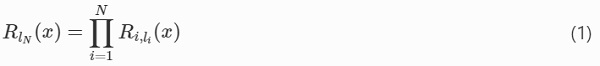
Strength modelling in glass tends to be based on either a Weibull weakest-link system, or the application of a standard statistical distribution such as a normal distribution (Weibull 1939; Calderone 1999). A weakest-link system is comprised of critical subsystems. The subsystem that is the weakest when the stresses are applied governs the failure of the entire system. This represents the condition of the glass surface which is brittle and presumably contains a large number of microscopic defects that limit the practical strength. With F(x) denoting the failure distribution function, R(x)=1−F(x) is the survival function which gives the probability that the system has not failed. The weakest-link scaling premise is expressed in Eq. (1) for a system consisting of N links where Ri,li(x) refers to the survival function of the i-th link with support in li while the system as a whole has support in lN (Hristopulos et al. 2015).
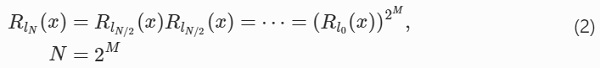
Weibull (1939) assumed that all the links have a common survival function with an exponential dependence and the Weibull distribution, Eq. (A.30), is the archetypical weakest-link scaling system. As expressed in Eq. (2), such a system has a self-similarity property which implies that except for a size scaling, the probability distribution for the survival of a system composed of any cluster of subsystems has the same functional form as the single-link survival function (Hristopulos et al. 2015).
Based on the same premise are, e.g., the Glass Failure Prediction Model in Beason and Morgan (1984) and the Lifetime Prediction Model in Haldimann (2006). In spite of the logical theory underpinning those WL-models, it remains a great challenge in general to predict the strength of a glass structure and according to some, there is no added benefit to safety prediction from the use of WL-systems compared to a normal or lognormal distribution (Calderone et al. 2001).
In reality, the computed probabilities of failure at the design stresses are only notional (Calderone and Jacob 2005), compare with the discussion in Annex A of EN 16612 (2019). It has been said that only a complex multiparameter model can describe glass test results widely in a single model (Veer et al. 2009). In the present study, a possible WL-framework for such a model is investigated, based on recent work by Yankelevsky (2014), Pathirana et al. (2017), Kinsella and Persson (2018), and Osnes et al. (2018).
Fracture mechanics
Surface flaws in glass are represented by cracks and the extension of a crack is modelled by an energy balance (Griffith 1920). Crack growth is prompted by either of three modes of deformation, viz. mode I, mode II and mode III (Irwin 1958). Mode I refers to crack opening due to displacements normal to the crack plane surfaces. Mode II and III describe in-plane and out-of-plane shearing displacement cracking (Broek 1983). As a simplification, only the impact of Mode I displacements are considered. Failure is governed by the critical release rate of elastic strain energy. The mode I stress intensity factor (SIF) for a sharp crack subjected to far-field tensile stress σ acting perpendicular to the crack plane is
![]()
where a is the crack size and Y is a geometrical configuration factor whose value is roughly equal to unity (Irwin 1957; Hellan 1984). For example, for a straight-fronted planar edge crack it is Y=1.12, and for a half-penny shaped crack it is Y=0.73 at the deepest point on the crack contour (Irwin 1958; Newman and Raju 1981). If the crack plane is inclined at an angle ϕ in the coordinate system of the principal stresses σ₁ and σ₂ with ϕ measured from the major axis, then the stress component acting perpendicular to the crack plane is calculated as
![]()
The fracture criterion is
![]()
where KIc is the fracture toughness.
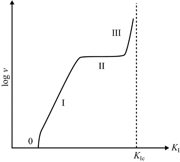
While subjected to tensile stress in an atmosphere that contains water moisture, environmentally assisted crack growth occurs in glass due to stress corrosion (Charles 1958a, b). The general shape of the logarithm of crack growth velocity as function of the magnitude of SIF is illustrated in Fig. 1. For structural glass design considerations, the influence of regions II and III on the time-to-failure can be neglected (Fischer-Cripps and Collins 1995). Subcritical crack growth in Region I is modelled using Eq. (6) in which v₀ and n are stress corrosion parameters and KI,th is a threshold value of SIF below which crack growth arrest occurs (Evans 1974). It is assumed that n=16 (Mencik 1992).
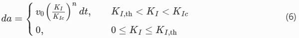
It can be shown that combining Eqs. (3) and (6) and introducing ai for the initial crack size and a(t) for time-dependent size after crack extension, the following equation holds (Haldimann 2006).
For the sake of interpreting laboratory tests at medium stress rate (including 2 MPa s⁻¹), Haldimann (2006) recommends the value v₀=10 μm s⁻¹, whereas a conservative assumption for design purposes is v₀=6 mm s⁻¹.
Tests
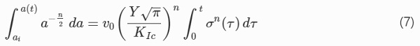
Tests were conducted on glass specimens subject to ring-on-ring and ball-on-ring bending using a hydraulic MTS uniaxial machine with a 10 kN load cell. In ring-on-ring bending, a plate is supported on a large ring on one side, and loaded through a smaller concentric ring on the other. A state of uniform biaxial tensile stress is produced within the centre part of the plate specimen bounded within the load ring radius on the rear surface. Beyond the load ring the tensile stresses diminish rapidly and edge failures are deemed unlikely (Simiu et al. 1984). The ball-on-ring configuration likewise depends on applying a load centrally, in this case through a steel ball. The maximum stress occurs at the centre where the radial and tangential components are equal. The bending rigs are illustrated schematically in Fig. 2. The ring-on-ring design was guided by ASTM C 1499-02.
Specimens with geometrical dimensions according to Table 2 were prepared from a single jumbo plate. The experiment involves monolithic annealed float glass panes that are new, in the as-received condition. The tests were performed in an ambient environment corresponding to an indoor climate. The average temperature and relative humidity during tests were 23°C and 50%. Two series of tests were conducted with the tin side of glass positioned in the tension zone. To facilitate a fractographic analysis of the fracture origin, the compression side of each specimen was covered in self-adhesive plastic foil prior to testing. Centre point displacement was measured using a linear potentiometer positioned directly below the specimen.
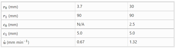
In Table 3, the geometrical dimensions and crosshead displacement rate, u˙, of the bending configuration are specified where the load ring and equivalent ball contacting radius (see App. A.2 for the determination of effective ball contacting radius), respectively, are denoted by r₀, the support ring radius by r₁, and the load and support ring cross-sectional radii by c₀ and c₁, respectively. The actual loading ball radius is 5 mm. The crosshead displacement rate was selected to produce an approximate stress rate of 2 MPa s⁻¹ at the centre point on the tension side.
Table 2 Geometrical dimensions of test specimens - Full size table
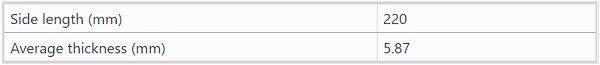
Table 3 Properties of bending setup - Full size table
The strain was measured on the tension side of two reference specimens at the centre point using a strain gauge rosette (HBM RY11 6/120), and at four symmetrically located points 25 mm away from the centre using linear strain gauges (HBM LY11 6/120) which were oriented parallel to the radial direction. These reference plates were subject to ring-on-ring and ball-on-ring ramp loading similarly to the specimens which were destroyed in strength tests. The values of recorded strain (in the principal directions) at the centre point, and the average value at the four symmetry points, respectively, were found to be within 1% of numerical predictions in a finite element analysis (see Sect. 4.1 for details about the finite element model).
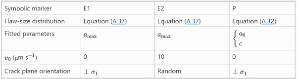
Table 4 Flaw-size concepts explained - Full size table
Modelling
In subsequent analysis, failure of the single-link is evaluated assuming that a given flaw has a representation as a crack (1) with a geometrical configuration, and; (2) with an orientation of the crack plane with respect to the stress field, and; (3) which is possibly operated on by stress corrosion producing time-dependent subcritical crack growth. In Lamon (2016), this notion of the physical processes taking place inside the link is referred to as a flaw-size based approach to fracture in contrast to an elemental strength approach which is not based specifically on a representation of flaws in terms of a crack. In the latter case, only the density function of elemental strengths is required as in, e.g., the Matthews et al. (1976) failure model. The value of plate thickness used in the stochastic failure modelling is equal to the average value recorded in Table 2.
Assuming an infinite-size weakest-link system, i.e. one with an infinite number of subsystems, the two-parameter Weibull distribution is derived by taking into account the correspondence between flaw size and macro-mechanical stress field according to linear elastic fracture mechanics. To determine theoretically the strength scaling due to a size effect in plates subject to biaxial loading, an effective area is calculated which represents a fictitious surface exposed to a uniform stress field. In the present study, this type of model is generated by a flaw-size concept which depends on a Pareto distributed flaw-size density. This approach is referred to by a symbolic marker ‘P’, see Table 4, and further details are given in Sect. 4.2.
Finite-size weakest-link systems are considered in numerical implementations with randomly generated cracks. The subsystems correspond with nodes on a rectilinear lattice and represent potential fracture sites. System failure is determined through a linear elastic fracture mechanics analysis based on the computed stress history which is obtained in a finite element analysis, see Sect. 4.1 for details about the finite element model. The fracture stress and failure origin are identified using a numerical procedure. In a large number of simulations, the statistical strength distribution is obtained for the respective bending setups.
The effect of stress corrosion is accounted for in the numerical computation method by implementing subcritical crack growth. In the present study, this type of model is generated by various flaw-size concepts governed by an exponentially decaying flaw-size distribution. This approach is referred to by symbolic markers ‘E₁’, ‘E₂’, etc, see Table 4. Concept ‘E₁’ corresponds basically with what was implemented in Yankelevsky (2014) whereas concept ‘E₂’ includes random crack plane orientation and an implementation of subcritical crack growth, further details are given in Sect. 4.3.
Finite element model
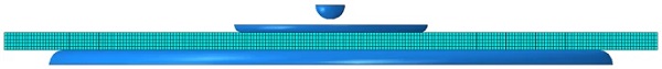
A static and geometrically non-linear finite element (FE) analysis is conducted to compute the bending stresses in a plate specimen using the commercial finite element code ABAQUS/CAE, see also Fig. 3. The elastic constants are adopted from Table 1. The self-weight is not included in the analysis. To model the glass part, an 8-node quadrilateral continuum shell element (SC8R) with reduced integration is employed in a structured mesh grid. The element size used in analysis is approximately equal to 1 mm with a total number of five through-the-thickness elements. The surface dimensions of the glass body are given in Table 2. The steel rings and ball are modelled by analytic rigid surfaces. The geometrical properties assigned to the analytic surfaces can be found in Table 3, and the ball radius used is 5 mm.
The parts are assembled and interaction surface-to-surface contact applied. It is assumed that frictional effects are negligible. The analytic surface representing the support ring is constrained to a reference point which is encastred. The analytic surface representing the load ring/ball is constrained to a reference point which is prevented from moving except in the lateral direction, and a concentrated force is applied to this reference point. To prevent rigid body motion of the glass part, it is constrained in the in-plane directions at a select number of symmetry points as follows. Let x, y be a Cartesian coordinate system with origin at the centre of the glass bottom surface and contained in its plane with axes parallel/orthogonal to the sides of the glass part. Then with L equal to the side length, for (x,y)=(±L/2,0) movement is constrained in the y-direction, and for (x,y)=(0,±L/2) it is constrained in the x-direction.
Infinite-size WL-system with Pareto flaws
The premise in Eq. (2) can be developed into a logical expression for the total failure probability of an infinite-size WL-system representing a surface area exposed to uniform stress σ in a state of uniaxial tension as in Eq. (8) (Wachtman et al. 2009).
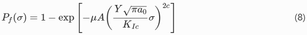
The basis for Eq. (8) is that (1) the average number of cracks, μA, is Poisson distributed, Eq. (A.34); (2) cracks fail independently of each other, and; (3) cracks are distributed over the surface according to a uniform random distribution with Pareto distributed sizes, Eq. (A.32), where a₀ and c are the Pareto scale and shape parameters, respectively. Equation (8) can be written in the form of the Weibull function (A.30) with,
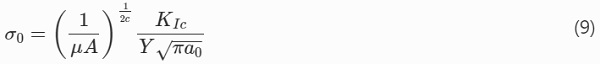
and,
![]()
When the tensile stress field is non-uniform and uniaxial, the total failure probability in Eq. (8) is rewritten as (Haldimann 2006),
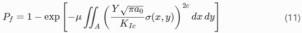
In a biaxial stress state, the greatest major in-plane principal stress, σmax, is introduced as parameter (Entwistle 1991). Rewriting Eq. (11) with this parameter, the distribution function for the strength is

where
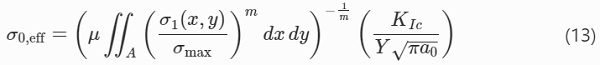
Here it is assumed that only the major in-plane principal stress component contributes to failure so that with the fracture criterion, Eq. (5), crack planes are always oriented perpendicular to σ₁. The original area, A, in Eq. (9) has been replaced in Eq. (13) by an effective area, Aeff, according to
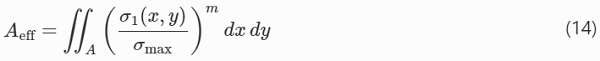
The strength-scaling effect when the flaw populations and environmental conditions are otherwise held constant is expressed as follows where σ₀,eff is the scale factor corresponding to Aeff and σ′₀,eff to A′eff, respectively.
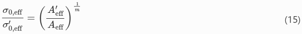
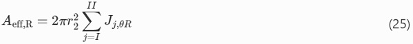
Equation (15) applies to the scale parameters only for two distributions which have equal shape parameters. The effective areas for plates subjected to ring-on-ring and ball-on-ring bending, respectively, are calculated using closed-form solutions for the stress which can be found in Appendix A.2. The major principal stress is given by σθ in Eqs. (A.40) and (A.47) for the ball-on-ring and ring-on-ring setup, respectively. The effective area, Eq. (14), is calculated using polar coordinates expressed in the normalized geometrical parameters, Eq. (A.38). After substituting for dr=r₂dρ it is,
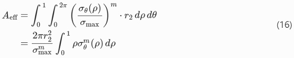
It is understood that the integral is performed only for those values of stress that are tensile. Accounting for the piece-wise expression for the ball-on-ring circumferential stress component in Eq. (A.40), the integral equation (16) can be written as a sum according to the solution in Frandsen (2014),
where fractions Jj,θB for j=I,II,III are as follows.
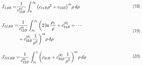
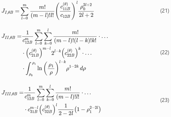
JI, JII, and JIII represent the contribution to the (normalized) effective area while 0≤ρ<ρ₀, ρ₀≤ρ<ρ₁, and ρ₁≤ρ≤1, respectively. Closed-form solutions to Eqs. (18) to (20) are given below on assumption of integer values of the Weibull modulus, because the multinomial theorem is used to handle the integration of multiple terms raised to the power of m (Frandsen 2014).
Also, the integral in the expression for JII,θB is
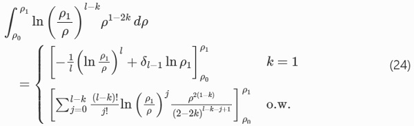
where δi denotes the Dirac delta function (Frandsen 2014).
In the case of the ring-on-ring setup, the piece-wise expression for the circumferential stress component in Eq. (A.47) is combined with Eq. (16) to produce the sum
The fractions Jj,θR for j=I,II for the ring-on-ring setup are obtained in analogy with the solution for the ball-on-ring case, after slight modification of the equations and replacement of integration limits.
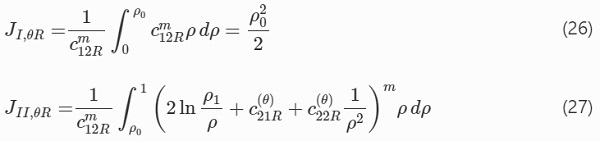
The closed-form solution to Eq. (27) is similar in form to Eq. (23) and is therefore not written out, compare with Eq. (19).
The strength-scaling is determined by substituting Eqs. (17) and (25) into Eq. (15). According to Eq. (15), this corresponds to the ratio of the 63rd percentiles in corresponding Weibull distributions (see also App. A.1). The Weibull parameters in Eq. (A.30) are estimated from experimental observations with the maximum likelihood method (Young and Smith 2005), where in practice the computations are performed using the wblfit function in Matlab. The corresponding Pareto flaw-size parameters in Eq. (A.32) can then be determined from Eqs. (10) and (13).
Numerical implementation of finite-size WL-systems
The surface area A of a jumbo sheet is represented by a uniform rectangular meshgrid, the nodes of which correspond to potential fracture sites. Only nodes that correspond to the surface area are considered so edge failures are neglected. Each node is located at the centre of a unit cell of some predefined size. In the present work, the cell size is 1 mm² and the spacing between the nodes is 1 mm in the longitudinal and transversal directions, respectively. An average number of N₀=μA cracks are uniformly distributed over the cells; the total number on a given plate is a Poisson random number with expectation N₀, Eq. (A.34). If a given cell contains more than one crack, then the largest one only is selected. An orientation is assigned to each crack with the angle uniformly distributed in [0,π). Each crack is assigned a size and shape according to some assumed distribution and geometry. Virtual specimens are extracted from the basic plate and analyzed as follows.
In a geometrically nonlinear analysis, the in-plane stress components, and time-variant mode I SIF, Eq. (3), are calculated at each crack-containing node and at a predefined number of time frames each of length Δt for i=1,…,Nt with Nt being the total number of time frames. The number of time frames is chosen large enough so that the maximum stress increase anywhere on the plate is smaller than approximately 0.1 MPa. Subcritical crack growth is calculated based on Eq. (7) with modified integration limits a(t) replaced by ai+Δa on the left-hand side, and t by Δt on the right-hand side. Also, to calculate the integral on the right-hand side of Eq. (7), the stress is linearized in each time frame.
Subcritical crack growth is allowed to occur only in time frames that correspond with a SIF that exceeds the threshold limit value, KI,th. Subsequently, the SIF history is adjusted to reflect the influence of subcritical crack growth. An algorithm is used to search through the SIF history for the first instance of a failed crack, fracture being governed by the criterion in Eq. (5). According to the weakest-link principle, failure of the specimen is deemed when the first crack fails. It is assumed that unit cells fail independently of each other. The strength is defined as the major in-plane principal stress at the failure node. However, because the SIF history is discretized, the time step associated with failure corresponds to a SIF equal to or larger than the fracture toughness. The strength is calculated by linear interpolation of the maximum principal stress at time steps before and after failure based on the corresponding SIF values.
The numerical method is implemented in a Python script that interfaces with (1) ABAQUS/CAE where a finite element analysis is carried out, and; (2) a Fortran program where an analysis of the weakest-link scaling system is performed. The Fortran program depends on a module for random number generation (Miller 2000; Blevins 2020). Strength statistics are obtained by running a series of tests on virtual specimens. The number of specimens that can be extracted from a single jumbo plate is limited. As one jumbo plate is exhausted, another one is sampled from which new specimens are subsequently extracted. Statistics are computed through repeated sampling from 14 base plates which in the present case (given the surface dimensions of each extracted specimen, see further Sect. 3) corresponds to over 5000 individual tests. This number is sufficient for convergence (Yankelevsky 2014).
The flaw-size concept that is implemented depends on a range of parameters, e.g., the flaw-size density function parameter(s). In the present work, a basic flaw-size concept is adopted from recent literature and analyzed, namely the approach suggested in Yankelevsky (2014), see below in the following subsection for a further description of this approach. This basic flaw-size concept, which is governed by an exponentially decaying flaw-size distribution, is denoted by a symbolic marker ‘E1’, see also Table 4. In addition, a flaw-size concept ‘E2’ is implemented in numerical analysis based on the exponentially decaying flaw-size concept ‘E1’ but with account for random crack plane orientations and including an implementation of subcritical crack growth. In order to fit the flaw-size concept to laboratory data, minor adaptations are made to the original model; specifically the flaw-size density parameter, amaxamax, in Eq. (A.36) is optimized.
Trial points for the parameter are set up and a goodness-of-fit statistic is computed at each one using a weighted measure of the distance from the empirical strength distribution function. The optimization procedure depends on selecting for the minimum of the Anderson-Darling two-sample statistic (Scholz and Stephens 1987). In practice the computations are performed using the andersonksamp function in the stats module of Python SciPy (Virtanen et al. 2020). To obtain a reasonable estimate while limiting the computational time, the resolution of the parameter space is restricted to values of one micron in the interval [0,300]μm. For reference, Yankelevsky (2014) supposes that a value of about amax=200μm would be representative, however this was not actually verified in laboratory tests. In addition to the flaw-size concept proposed in Yankelevsky (2014), see also Pathirana et al. (2017) and Kinsella and Persson (2018) for examples of other approaches which apply both single and multiple flaw-populations that co-exist on a given surface.
The numerical implementation does not directly lead to a closed-form expression for the strength-scaling similar to Eq. (15). However, the 63rd percentiles in the computed strength distributions can be determined and their ratio calculated to produce a measure of size-effect comparable to Eq. (15).
Flaw-size approach in Yankelevsky (2014) The straight-fronted edge crack shape is adopted by Yankelevsky (2014) with an exponentially decaying size distribution that is parametrized by the size of the largest crack, amax, that is present in the population, see Eq. (A.37). It is assumed that for new glass in the as-received condition, a representative value is 1 flaw per square centimetre density. It is claimed that with this model, there is no need for calibration because it is independent of test results. Only the maximum crack size that is present in the population is required as input and this number can be inferred from the standards, e.g. EN 572-2 (2012), and the fact that manufacturers inspect the glass for large defects. Subcritical crack growth is not considered and all crack planes are assumed to be oriented perpendicular to the major in-plane principal stress.
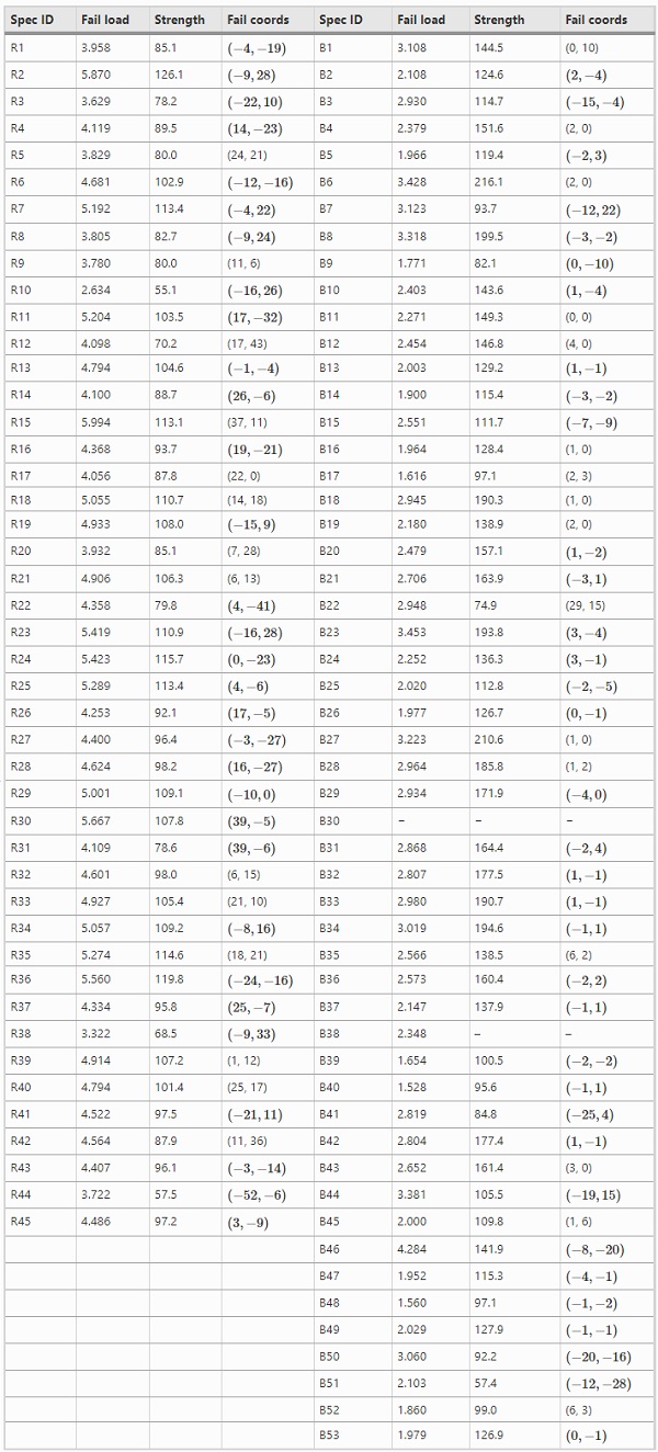
Table 5 Recorded failure load (kN), computed strength (MPa), and recorded fracture coordinates (mm) as measured from the centre point of the plates in laboratory tests - Full size table
Results
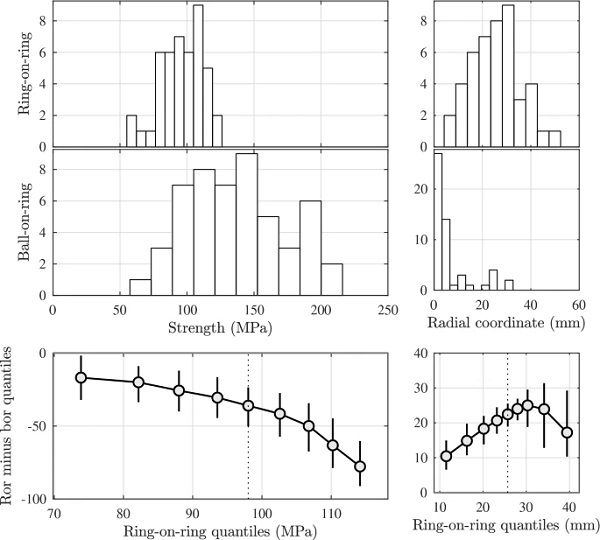
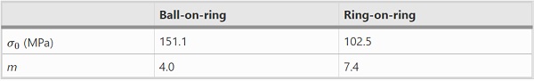
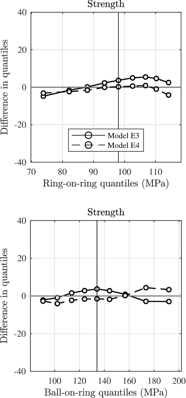
Table 5 lists the failure load, strength, and recorded fracture origin from the conducted experiments. The given strength value is the major in-plane principal stress component at the fracture origin, computed according to a FE analysis. For specimen B38, only a fracture load is given because it disintegrated prior to examination and a precise fracture origin could not be established. Specimen B30 was by mistake positioned upside down in the apparatus with the self-adhesive plastic foil on the tension side, thus invalidating the result. In Fig. 4, the computed failure stresses and recorded fracture origins are displayed in histograms. The difference in estimated quantiles between the data sets is also illustrated in the figure using the Shift function which is described further in Appendix A.3. For each decile in the shift function, a vertical line indicates its 95% confidence interval obtained using a bootstrap method, see Rousselet et al. (2017) for a further description. Estimated Weibull parameters are given in Table 6 for the laboratory strength data samples.
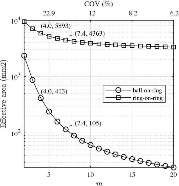
Figure 5 shows the calculated effective area as function of Weibull modulus according to Eqs. (17) and (25). The correspondence between Weibull modulus and COV according to Eq. (A.31) is indicated on top of the diagram in Fig. 5. The effective areas at the estimated values of Weibull moduli (found in Table 6) were calculated using linear interpolation where so necessary and are specified in the figure.
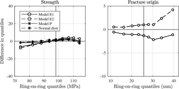
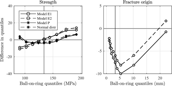
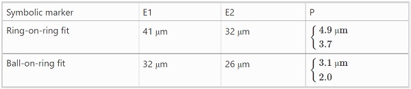
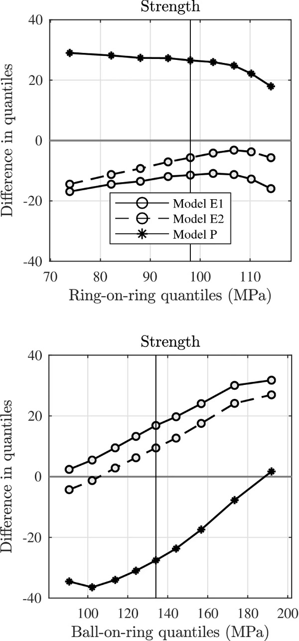
Figures 6 and 7 compare the quantiles in the laboratory data samples with a range of models that are fitted to the ring-on-ring and ball-on-ring strength data, respectively. The fitted models include (1) a Weibull distribution, Eq. (A.30), and; (2) a normal distribution, Eq. (A.33), and; (3) numerical implementations of finite-size weakest-link systems governed by different flaw-size concepts. The flaw-size concepts are explained in Table 4 and the fitted flaw-size distribution parameters are given in Table 7. The flaw-size concept denoted by ‘P’ corresponds to the Pareto flaw-size distribution which generates the Weibull strength model as described in Sect. 4.2.
The flaw-size concepts denoted by ‘E1’ and ‘E2’ correspond to an exponentially decaying flaw-size distribution used in numerical strength modelling with finite-size weakest-link systems as described in Sect. 4.3. The Pareto flaw-size parameters, Eq. (A.32), that correspond to the fitted Weibull distributions are inferred by substituting the values from Table 6 into Eqs. (10) and (13). When stress corrosion is accounted for in numerical simulations, it is assumed that the applied loading rate is such that a 2 MPa s−1−1 stress rate occurs at the centre point on the tension surface.
Figure 8 presents a comparison of the experimentally recorded quantiles with strength predictions made from the fitted models. Hence, the models fitted to the ring-on-ring strength data in Fig. 6 are used to make predictions for the ball-on-ring setup as shown in Fig. 8, and the models fitted to the ball-on-ring strength data in Fig. 7 are used to make predictions for the ring-on-ring setup. The predicted Weibull distributions depend on the calculated effective areas shown in Fig. 5, which are substituted into Eq. (15) while assuming a uniform value for the Weibull modulus. Hence, when Weibull predictions are made for the ball-on-ring setup it is the estimated modulus from the ring-on-ring case that is used, and vice versa.
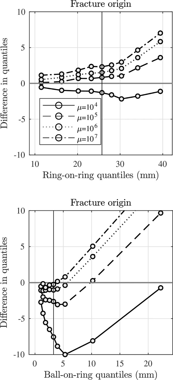
Figure 9 illustrates how the distribution of fracture origins depends on the assumed value of flaw density μ in the range 10⁴ to 10⁷. The flaw size concept that was chosen to render the figure is otherwise the same as E1 in Table 4.
The tests also provide information about the stiffness of the glass material. Young’s modulus E can be calculated using Eqs. (A.51) and (A.52) which express the centre-point displacement as function of applied load. The observed values of load and displacement in laboratory tests inserted into those equations give an average of about E=69.6 GPa. This is close to the nominal value given in Table 1 and therefore this value was used in the present investigation.
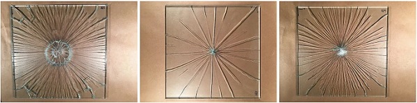
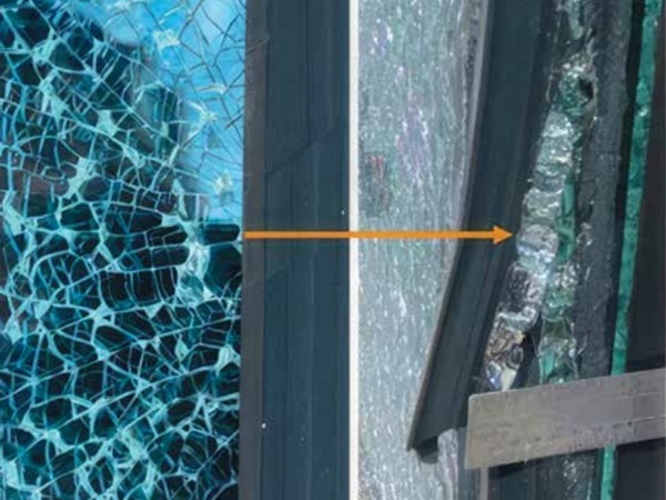
Figure 10 shows the broken specimens no. R13, B29, and B39, respectively, which exhibit representative fracture patterns.
Table 6 Weibull distribution parameters fitted to strength test results - Full size table
Discussion
Weibull systems
Both the Weibull and normal distribution provide a basic strength model that is in close agreement with the ring-on-ring and ball-on-ring laboratory test results. In fact, their performance as a strength model is more or less equal and from a pragmatic point of view only, neither can be deemed better than the other, compare Figs. 6 and 7. From a theoretical perspective, the Weibull model has the quality of being founded in a flaw-size based WL-system which is logical in application to glass considering the underlying physical processes which are supposed to prompt fracture. Indeed, the Weibull modulus can be given physical meaning as a material parameter (De Jayatilaka and Trustrum 1977). The Weibull model’s foundation in a WL-system implies a well-defined strength-scaling effect which is a function of the size of surface area exposed to tension.
In the laboratory tests on nominally identical glass specimens that were conducted as part of this study, however, the estimated Weibull modulus was observed to vary considerably between test setups using a pair of biaxial bending configurations. Hence, the self-similarity property at the core of the WL-scaling premise in Eq. (2) is contradicted. Prediction of the ball-on-ring (ring-on-ring) strength based on the Weibull effective area, Eqs. (17) and (25), produces a considerable overestimation (underestimation) when based on a model fitted to the outcome of ring-on-ring (ball-on-ring) bending, see Fig. 8. In summary, even though the Weibull model has descriptive virtue, there are limits to its predictive capacity and potential for use in design rules.
Table 7 Fitted parameters of flaw-size concepts - Full size table
Considering the histograms in Fig. 4 and the adjacent shift function for the laboratory test results, it is strongly suggested that surface size effects in glass are not only a matter of strength scaling. It is indicated that the shape of the distribution changes, too, however this is more apparent in the high-strength domain (right-hand tail) than it is for quantiles below the median. In other words, the right tail shifts more than the left, and the ball-on-ring test data displays a larger spread in the distribution of medium to high-strength specimens. It is worth noting in this context that there exist variants of the ordinary Weibull model that represent finite-size WL-systems that do not obey the self-similarity property in Eq. (2) and yet are expressed in closed-form.
The κ-Weibull distribution is an example of this and it has a tail that decays like a power-law in contrast with the usual Weibull distribution’s exponentially decaying tail (Hristopulos et al. 2015). The κ-Weibull distribution lies beyond the scope of the present investigation because its foundation in a strict flaw-size concept is not evident like with the ordinary Weibull distribution. However, it may be worth exploring in future work. An applied normal distribution is not associated with a flaw-size based WL-system, and hence the typical notion of WL-scaling or indeed fracture mechanics does not find a direct application. This is a drawback from a theoretical point of view. At least this has the benefit that results are taken at face value (Gorski 1969).
Finite-size systems
Two types of finite-size weakest-link systems are implemented numerically and are governed by an exponentially decaying flaw-size distribution, see Table 4. With each one, it is possible to obtain a reasonable agreement with the laboratory strength results. The tendency is for the spread in the strength distribution to get slightly underestimated, in particular with the fitted ball-on-ring models, as suggested by the sloping curve of the shift function (Fig. 7). When predictions are made of ring-on-ring strength from the ball-on-ring outcome, the location is shifted in the distribution and the median strength gets overestimated slightly (Fig. 8). Predictions of ball-on-ring strength exhibit a clear lack of spread compared to laboratory test results and produce an underestimated median strength.
Considering the strength predictions in Fig. 8, it should be noted that the Weibull distribution gives the opposite effect in terms of under/overestimation compared to the numerical analysis with finite-size WL-systems, namely, when the Weibull distribution underestimates the strength in predictions of ring-on-ring bending, the numerical simulations slightly overestimate, and vice versa for the ball-on-ring predictions. Notice, however, that in terms of the median and lower quantiles, which are the most important in design considerations, the numerical simulations tend to perform better than the Weibull distribution, as these produce predictions for the quantiles that are located closer to the estimated values observed in experimental strength tests.
The fitted flaw-size distribution parameters in Table 7 are considerably lower than suggested in Yankelevsky (2014), compare Sect. 4.3. This presents a problem to the physics-based interpretation of the parameter amax in Eq. (A.37). The argument may not be viable that this parameter value can simply be inferred from standard documents with quality requirements, e.g., on the largest optical fault as new glass is inspected for large defects by manufacturers, because that would suggest a higher value than what is recorded in the table, compare with the line of reasoning in Yankelevsky (2014) and also Pisano and Royer-Carfagni (2017). Additionally, with the values of amax recorded in the table, the strength in numerical simulations (without implementation of subcritical crack growth) would never fall below about 55 MPa, compare Eq. (3), irrespective of how much the surface area were increased that is exposed to tension, and this seems to be unrealistic and a severe drawback from a practical point of view.
Taking into account also the modelled and predicted failure origins, it is evident that the numerically simulated WL-systems perform better for the ring-on-ring than for the ball-on-ring setup. In the ball-on-ring laboratory tests, most of the observed fracture origins occurred close to the centre, within a radial distance of about 5 mm. In contrast, with the numerically simulated weakest-link systems, the proportion of fracture origins located nearest the centre is considerably underestimated, compare Fig. 7 which shows that the median value of radial coordinate is shifted away from the centre by 5–10 mm.
The same can be seen (in Fig. 8) when predictions are made on the ball-on-ring setup from a model originally fitted to the ring-on-ring setup. In addition, the same feature in the ball-on-ring fracture origin distribution as already mentioned is also obtained when a flaw-size distribution with power-law decay is implemented in numerical simulations of finite-size systems, and hence the feature is observed for all of the different types of flaw-size concepts recorded in Table 4. The surface condition may not be represented accurately enough in the flaw-size concepts.
For example, the assumed flaw density may be too low. From a practical point of view, there is limited knowledge about the true surface condition in glass because surface flaws are hard to detect using current technology and ultimately recourse has to be made to elementary assumptions. There have been recent attempts to probe flaws non-destructively using image scanning techniques (Wereszczak et al. 2014), however it remains to be demonstrated that such methods are capable of detecting all pertinent flaws and to distinguish potential fracture-inducing flaws from other less severe ones (Lamon 2016).
For the ball-on-ring setup, Fig. 9 shows that by increasing flaw density, the fracture origin spread in radial direction is reduced with a shift towards the centre which generally reflects the empirical ball-on-ring data set better. At the same time, with increased flaw density, it is possible that spurious fractures that occur at a greater distance from the centre-point get underestimated. With the ring-on-ring fracture origin distribution, a slight shift occurs in origin location towards the centre as flaw density increases, and, the right-hand tail gets diminished. It should be noted that there is much greater uncertainty in the decile estimates of the right-hand tail of the fracture origin distribution than in the left-hand tail, compare with Fig. 4 which shows the shift function with confidence bounds for the laboratory test data samples.
For 10⁴≤μ≤10⁶ in both ring-on-ring and ball-on-ring loading, the confidence bounds (not shown in Fig. 9) for the 8th decile in fact cover the value zero. In addition, by increasing the flaw density while using the chosen flaw size concept from Table 4, the spread in simulated strength distribution (not shown in Fig. 9) gets severely reduced to the point of rendering the strength model ineffective. Therefore, it is not possible to directly reconcile the observed strength and fracture origin distributions for the ball-on-ring setup in numerical simulations by increasing the flaw density value alone.
The significance is emphasized of taking into account not just the recorded fracture stresses in weakest-link analysis of glass strength, but also fracture origins which for logical reasons are intrinsically interconnected in such systems. In fact, the simultaneous modelling of strength and fracture origins is easily overlooked in casual fitting of a Weibull distribution to brittle strength data. Even though it is intuitively compelling to represent flaws as cracks (with geometrical configuration, directional sensitivity to the applied stresses, etc.), it may not be the most expedient way to proceed in a weakest-link framework. For example, the definition of crack geometry is straight-forward whereas in reality a flaw may have a complex shape (Lamon 2016).
Table 8 Modified flaw-size concepts explained - Full size table
Modified flaw-size concepts
Figures 6, 7 and 8 suggest a number of basic problems that arise with the use of the flaw-size concepts from Table 4, namely: (1) models based on these concepts are not altogether capable of predicting the results from one setup based on the outcome of another; (2) considering the E-type concepts from Table 4, the fitted values of amax are so small as to cause too low a limit on the possible flaw-size than is practical; (3) the spread in fracture origins for ball-on-ring bending gets considerably overestimated.
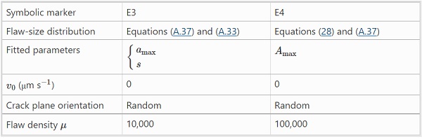
To address the first two issues mentioned above, a pair of modified flaw-size concepts are proposed in Table 8. The first one, E3, addresses the issue relating to the capacity for using the results from one bending configuration to predict the outcome of another. It relies on adding a small random noise to each unit cell after the Griffith flaws have been sampled and distributed across the surface. The random noise is assumed to be normally distributed with mean zero and standard deviation s, Eq. (A.33).
A physics-based interpretation of the random noise involves the compounded effect of various phenomena acting locally, such as complex flaw shapes that take on random geometrical configurations, presence of residual stresses over the surface with local deviations, and other random effects that arise as a consequence of interaction between the surface and its surroundings. In reality, such random noise could be correlated in space, with neighbouring unit cells potentially displaying stronger correlation; however, as a simplification this is disregarded.
The second modified flaw-size concept, E4 in Table 8, depends on adopting a doubly stochastic flaw-size distribution in the form of allowing amax to display random variability. The reasons for viewing amax as a random variable include: (1) unless the glass surface is artificially damaged, e.g., through abrasion (Blank 1993), it is unlikely that failure is governed by a single flaw population. Random variability in amax allows for a multitude of flaw populations to be represented, all the while maintaining the underlying exponential dependence that is expressed in Eq. (A.35); (2) it enables a shift in the flaw-size distribution towards smaller flaws without destroying the possibility for rare occurrences of a large flaw. As a model for the random variability in amax we consider the model expressed in Eq. (28) which is the same as in Eq. (A.37) but with substituted variables,

and, where Ni is determined according to Eq. (A.37), see further App. A.1. Hence, it is assumed that amax is a positive random number smaller than some upper limit, Amax, equal to say 200 μm, and that it has an exponential decay. When the Griffith flaws are sampled in the numerical procedure, a value for amax is first sampled using Eq. (28) based on the fixed parameter value Amax, and subsequently inserted into Eq. (A.37) to draw a random flaw size which is then assigned to a unit cell. The reason for adopting this particular stochastic model for amax is: (1) it is a simple model that does not introduce additional parameters into the system, and it also retains the functional form already present; (2) it readily shifts the sampled flaw sizes to much lower values without destroying the possibility for very large flaws to occur, however, rarely. Notice, that because of this shift in flaw sizes, it may be expected that the associated flaw density, μ, requires additional adjustment.
Table 9 Fitted parameters of modified flaw-size concepts - Full size table
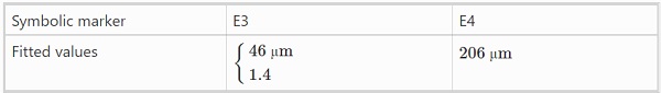
Table 9 shows the fitted values of amax and s, and Amax and μ, respectively. The fitting was performed through trial and error; in the case of E3 by starting out from a value of amax in the neighbourhood of those already recorded in Table 7, and adding to this a small random noise with standard deviation approximately equal to one micron; in the case of E4 by starting out from a value of Amax at about 200 μm (which would preserve this parameter’s physics-based interpretation as the globally largest flaw size present in new glass in the as-received condition, compare with Yankelevsky (2014)), and then increasing the flaw density suitably. For sake of simplicity, subcritical crack growth is neglected in the modified flaw-size concepts.
The addition of a small random noise leads to a fit with the respective data sets which simultaneously allows for prediction-making of one setup based on the outcome of the other, see Fig. 11. The confidence bounds for the quantiles (not shown in figure) suggest that the fit is within statistical reproducibility. With the use of the doubly stochastic flaw-size concept, a satisfactory fit with the ring-on-ring and ball-on-ring data sets is also produced simultaneously, while at the same time maintaining a large enough value of Amax for the preservation of its physical interpretation.
In fact, with the value Amax=200μm a fit is just about obtained within statistical reproducibility (as per the confidence bounds of the quantiles) thus suggesting that this value can be recommended as a rule of thumb. The condition for this is that the flaw density is increased one order of magnitude from the original value in Table 7. However, the modelled fracture origins (not shown in figure) exhibit the same kind of features as previously shown in Figs. 6 and 7, viz. the ring-on-ring origins are modelled reasonably well whereas the spread in ball-on-ring origins is considerably overestimated.
It should be noted that while the WL models E3 and E4 show better results than the ordinary two-parameter Weibull distribution, a three-parameter Weibull model would also show better results compared to the two-parameter Weibull distribution because of the increased number of parameters used in the model fitting.
Low-strength prediction
As the laboratory test samples are somewhat limited in size (≈50), it is hard to estimate with reasonable accuracy the behaviour of quantiles beyond approximately 0.1 and 0.9 (see also App. A.3). If the fitted strength models are used to make extrapolation, the following should be noted. The left-hand tail of fitted Weibull and normal distributions is larger than for the numerically simulated WL-systems. This means that predictions of low-strength quantiles are most conservative with a Weibull or normal distribution. This is not surprising because the flaw-size concept that was implemented in numerical simulations involves a truncated exponential-type distribution, compare Eq. (A.37).
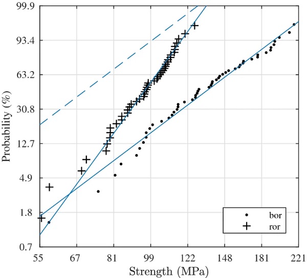
What would the left-hand tail in the ball-on-ring data set look like if a much larger number of laboratory tests were carried out? Such a question is relevant for strength design purposes. The ring-on-ring data set could in principle provide information about this, when it is considered that the calculated effective area represents a fictitious surface exposed to uniform tensile stress. In fact, rather than to increase the sample size, Danzer et al. (2007) proposes to test specimens of varying sizes to probe a greater range of the underlying flaw-size distribution. Given a data set of N observations of the strength, the estimate of the failure probability for a specimen is based on its rank in ascending order. The failure probability associated with the i-th specimen can be calculated using the Median rank estimate as follows (Forbes et al. 2011).

The values of Fi are located along the ordinate in a probability plot, compare with Fig. 12 which shows the Weibull plot for the ball-on-ring and ring-on-ring samples. In addition, a reference line (dashed line) is shown in the figure that represents a prediction for the strength distribution based on the ball-on-ring outcome when the effective area is increased by a factor 5893/413≈14 (compare the values of effective area in Fig. 5). According to this Weibull weakest-link model, one observation of ring-on-ring strength corresponds effectively to the minimum value of ≈14 number of ball-on-ring tests. Using Eq. (29), the lower quantile that is probed when the minimum value is selected from a sample of 14 observations is close to the 5%-fractile (compare also with Danzer et al. (2001)).
Another interpretation of the effective area pertains to the minimum value in the set of 45 ring-on-ring observations which would represent the minimum value in a set of about 45⋅14=630 ball-on-ring observations, a sizeable set of data. It is noteworthy that the minimum observed strength in the ring-on-ring data set (55.1 MPa) is only about 4% smaller than the correspondingly smallest observed value in the ball-on-ring data set (57.4 MPa), see Table 5.
In summary, a number of conclusions are conceivable. (1) The calculated effective areas are incorrect, e.g., the effective area in ball-on-ring bending is in reality much greater; (2) the Weibull function fitted to the ball-on-ring data cannot be used to model correctly the distribution of the (for example) 5% fractile which in such case produces overly conservative estimates for the strength; (3) there is in reality some sort of correlation between subregions/“links” in the WL-system which renders comparisons between the two biaxial configurations intractable when using standard (Weibull) WL-theory; (4) the underlying flaw-size distribution that generates the observed strength samples is in reality multimodal.
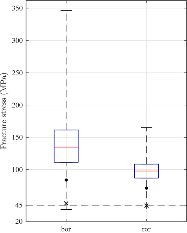
The boxplots and added features in Fig. 13 provide a visualization of summary statistics for the estimated median and low-strength quantiles from simulations with finite-size systems using the flaw-size concept E4 from Table 8. A number of 100,000 virtual tests were conducted to generate the displayed statistics. The line in the middle of each box is the sample median. The top and bottom of each box are the quartiles of the sample. The dot below the box represents the estimated 5%-fractile and the cross below it represents the 1 in 10,000 failure probability. The horizontal line at the bottom and top of each whisker extends to the minimum and maximum values in each data sample.
The dashed horizontal line near the bottom of the diagram indicates the 45 MPa characteristic value for the bending stress that is mentioned in EN 572-1:2012, and which is further discussed in an annex to EN 16612 (2019). From Fig. 13, it can be concluded that with the adopted model for the tested glass, the material is considerably stronger than the 45 MPa characteristic value mentioned in the standards. In addition, the 5%-fractile value decreases from about 84.0 MPa in ball-on-ring loading to 71.3 MPa in ring-on-ring, corresponding to a 15% strength decrease. It should be noted, that the 1 in 10,000 failure probability is roughly equal to 45 MPa in either loading case. In reality, with much larger structures spanning several metres and exposed to bending load, it may be that the size-effect is differently pronounced. More testing and numerical modelling is required to verify this.
Stress corrosion and flaw randomness
Implementation of stress corrosion can have a profound impact on the estimated flaw-size distribution parameters, depending on the chosen value of v₀ in Eq. (7). Unfortunately, the data on the crack velocity parameter, v₀, exhibits a large scatter, see e.g. Haldimann (2006) and Schula (2015) for a review of this. To simply adopt a conservative value for v₀ is problematic for a correct interpretation of the derived flaw-size distribution parameters in the numerical simulations. There is a need for more reliable information about the crack velocity parameter that can be used in modelling of tests performed in ambient conditions.
The location and orientation of flaws may in reality not be uniformly random distributed. The assumption that all crack planes are oriented perpendicular to the major in-plane principal stress is conservative. In reality, due to e.g. machining operations, there may be some preferred flaw orientations. In the present case with ring-on-ring and ball-on-ring bending, the in-plane principal stresses are equal at the centre point where the greatest tension arises. It is expected that the choice of crack plane orientation (uniform random or perpendicular to the major principal stress) has a limited impact on these results only. However, in other cases such as with four-point bending tests, the impact would be more significant.
Fracture patterns
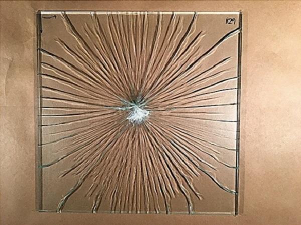
Figure 10 illustrates some of the observed fracture patterns in the broken specimens. The ring-on-ring plates typically display circumferential cracking occurring near the inner loading ring which indicates that the specimen strength was moderate to high (Quinn 2016). In addition, the circumferential cracking is likely exacerbated near the load ring because the suspended and approximately 11 kg heavy load jig weighed down on the broken specimen upon failure thus causing increased fracturing locally. A visual inspection of the broken ball-on-ring specimens reveals that the typical fracture pattern was a star-like one. “Star” cracking initiates on the rear tension side of the plate from a flaw which immediately bifurcates to produce a multitude of radial cracks which give a star-like appearance (Ball and McKenzie 1994).
In principle the number of radial cracks is proportional to the stress (Shah and Aung 2014). The failure load of specimen B29 is about twice as large as that of B39 and indeed the number of radial cracks is substantially greater. Basically, there are two stress systems in a ball-on-ring bending situation that compete with each other to produce the failure origin, namely Hertzian indentation stresses and bending stresses (Ball and McKenzie 1994). In the present case with relatively thin specimens that are simply supported on a large-diameter ring and subject to quasi-static loading, it is the bending stresses that govern failure with “star” cracking as a result. However, for thicker plates on a smaller ring, and/or with dynamic loading, failure may be prompted by a cone fracture that propagates through the thickness.
Conclusions
The theoretical strength-scaling in glass plates subject to ring-on-ring and ball-on-ring loading can be determined, on the basis of a Weibull weakest-link system, using the calculated effective areas which are expressed in closed-form. The so predicted strength-scaling is greater than the measured size effect in laboratory tests on new annealed soda-lime glass plates. In fact, the estimated Weibull modulus is found to vary considerably between the ring-on-ring and ball-on-ring experiments, thus rendering intractable the weakest-link scaling premise of the Weibull distribution.
Numerical implementations of finite-size weakest-link systems are carried out with flaw-size distributions that decay as an exponential function. These systems can provide more viable predictions for the strength-scaling compared to a Weibull distribution. According to this modelling, the characteristic 5%-fractile bending strength of the glass is considerably greater than 45 MPa. However, the simulated ball-on-ring fracture origins exhibit greater spread in the radial direction from the centre point compared to laboratory observations. This indicates that the surface condition representation considered in this work may not be properly configured to model all fracture origins, even though it is possible to make reasonable predictions for the statistical distribution of origins in ring-on-ring loading. The choice of stress corrosion parameter value can have a profound impact on the simulated results and the modelling of subcritical crack growth is important to address in future work.
There is a need for more insight into the surface condition of glass which can be conducive to the development of flaw-size based weakest-link modelling. Nevertheless, computationally intensive procedures for implementation of finite-size weakest-link scaling systems are likely conducive to the development of improved modelling tools compared with the basic Weibull distribution.
References
Acknowledgements
The following persons are gratefully acknowledged: Jessica Dahlström for valuable assistance with the experimental tests, Marcin Kozlowski for practical advice given in connection with the experiments, Johan Lindström for generous support in matters of statistical analysis, and Henrik Frandsen for constructive advice.
Funding
Open access funding provided by Lund University.
Author information
Authors and Affiliations
Division of Structural Mechanics, Faculty of Engineering LTH, Lund University, P.O. Box 118, 221 00, Lund, Sweden - David Kinsella & Erik Serrano
Corresponding author
Correspondence to David Kinsella.
Ethics declarations
Conflict of interest
On behalf of all authors, the corresponding author states that there is no conflict of interest.
Appendix
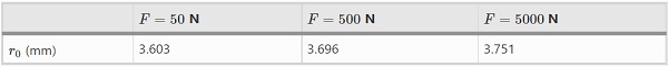
Table 10 Equivalent radius of contact between loading ball and specimen at various magnitudes of applied load - Full size table
Closed-form solutions for stress
The small displacement solutions for the stress distribution are derived assuming elastic bending of a rigid circular plate and considering only the bending stresses. It is assumed that the contact between the plate and ring/ball is ideally elastic and that the compliance of the test system is small relative to that of the test specimen. The radial and circumferential stress components are denoted by σr and σθ. The contact radius between ball and specimen can be calculated using Hertz’ elastic contact theory, however the contact stress directly under the ball is not homogeneous (Le Bourhis 2008). Instead, an equivalent radius of uniform loading is adopted and substituted in the closed-form solutions for the stress, Eq. (A.40).
The effective radius of contact between loading ball and specimen where the loading can be considered uniform is in the general case difficult to determine (Chae et al. 2010). The equivalent radius of uniform loading for the present ball-on-ring configuration was determined by comparing the analytical solution for centre-point stress on the bottom of the plate with FE-computations. The value of r₀ was chosen such that the corresponding maximum tensile stress under the plate using Eq. (A.40) is in close agreement with a FE analysis. The equivalent radius varies by about 1% within the range of load magnitudes that prompt failure in the tests. Table 10 shows the distribution of equivalent r₀ as function of load magnitude for the ball-on-ring configuration at a select number of points in the load history.
The normalized geometrical parameters are

where r₂ is the radius of a circular disk specimen. For a square plate with edge length L, the effective circular radius can be approximated as one half times the average value of the plate diagonal and side-length, i.e.,

The following ball-on-ring formulae were obtained from Frandsen (2014), and the expressions for ring-on-ring bending were obtained from Shetty et al. (1980) who developed the original solution by Vitman et al. (1962). The circumferential and radial stress components are expressed in terms of the normalized geometrical parameters on a general form with i={θ,r}. In the case of ball-on-ring bending, the equations are as follows where the subscript B refers to the ball-on-ring setup.
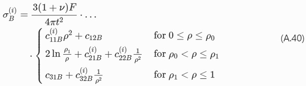
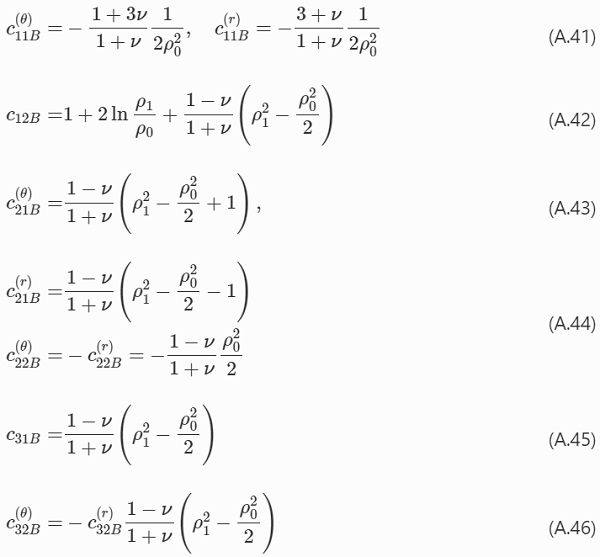
The constants in Eq. (A.40) are the following.
For the ring-on-ring configuration, the following equations are used where subscript R signifies the ring-on-ring type.
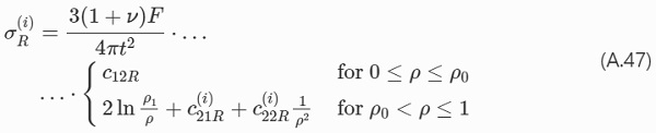
The constants in Eq. (A.47) are the following,
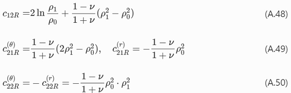
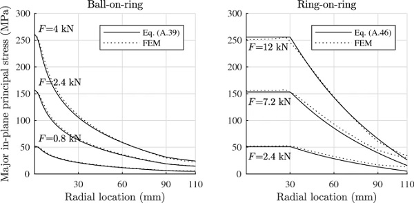
Figure 14 compares the calculated major in-plane principal stress in the radial direction from the centre point at three values of load for the ring-on-ring and ball-on-ring bending configuration, respectively, with FE-computations.
The centre-point displacements are, respectively (Vitman et al. 1962; Frandsen 2012),
Shift function
The shift function provides a tool for systematic group comparisons that combines a graphical method for comprehensive data visualization with robust inferential statistics and is further described in Rousselet et al. (2017). The shift function is a plot of the difference between the quantiles of two distributions as a function of the quantiles in one group. The quantiles are estimated and 95% confidence intervals are computed for the quantile differences. The shift function describes how much one distribution must be shifted or re-arranged to match another.
For example, two distributions that differ only in location would in principle produce a shift function in the form of a horizontal line displaced from the origin in the vertical direction. Whereas, two distributions that differ only in spread would produce a shift function in the form of a sloping straight line. Small sample sizes can pose a problem when addressing the question of how two distributions differ. According to Rousselet et al. (2017), it is recommended that at least 30 observations be included in an analysis to compare the 0.1 or 0.9 quantiles. 20 observations appear to be sufficient to compare the quartiles, i.e. the 0.25 and 0.75 quantiles. At least 50 observations per group should be used to compare the 0.05 and 0.95 quantiles.


")