Analytical Fragility Curves for Seismic Design of Glass Systems Based on Cloud Analysis

Author: Silvana Mattei and Chiara Bedon

Source: Symmetry 2021, 13(8), 1541; MDPI

DOI: https://doi.org/10.3390/sym13081541

(This article belongs to the Special Issue Symmetry Applied in Special Engineering)

Abstract

Given the growing spread of glass as a construction material, the knowledge of structural response must be ensured, especially under dynamic accidental loads. In this regard, an increasingly popular method to probabilistically characterize the seismic response of a given structure is based on the use of “fragility” or “seismic vulnerability” curves. Most existing applications, however, typically refer to construction and structural members composed of traditional building materials. The present study extends and adapts such a calculation method to innovative structural glass systems, which are characterized by specific material properties and expected damage mechanisms, restraint details, and dynamic features.

Suitable Engineering Demand Parameters (EDPs) for seismic design are thus required. In this paper, a major advantage is represented by the use of Cloud Analysis in the Cornell’s reliability method, for the seismic assessment of two different case-study glass systems. Cloud Analysis is known to represent a simple and immediate tool to analytically investigate a given (glass) structure by taking into account variations in seismic motions and uncertainties of structural parameters. Such a method is exploited by means of detailed three-dimensional (3D) Finite Element (FE) numerical models and non-linear dynamic analyses (ABAQUS/Standard).

Critical issues and typical failure mechanisms for in-plane seismically loaded glass systems are discussed. The validity of reference EDPs are addressed for the examined solutions. Based on a broad seismic investigation (60 records in total), fragility curves are developed from parametric results, so as to support a multi-hazard performance-based design (PBD) procedure.

1. Introduction

Recently, the rising sector of structural glass has been seen as a solid background for load-bearing components and building structures in general [1,2]. Both developments in the production processes and the continuous research innovation supported the safe structural use of this material in load-bearing elements, and its optimal combination with other materials such as wood [3,4,5,6,7], aluminium and steel [8,9,10,11], or composites [12,13,14]. According to current technical knowledge, the construction of columns, beams, walls, floors, roofs, and even stand-alone systems with load-bearing functions for glass is nowadays allowed. However, major safety issues in design relate to robustness, redundancy, ductility, durability, and even comfort [15]. Given the characteristic brittle behaviour of this material, when designing structural glass system, it is necessary to identify all the aspects involved in the response which results in an expensive calculation model, especially in case of seismic action [16,17,18,19].

In particular, thanks to the aesthetic appeal, facade systems became very popular since the early 1900s as enclosures for multi-storey buildings [20,21]. Therefore, the widespread use of glass walls since 1960 catches the interest of researchers on the behaviour of non-structural elements during seismic events, in order to prevent human and economic losses [22,23,24]. Recently, Caterino et al. [25] pointed out some major observations and results from earthquake surveys about the failure of non-structural components for buildings [26], and calibrated a set of detailed FE models for full-scale aluminium/glass curtain wall units. The validation of these models throughout experimental tests was used to numerically predict the in-plane lateral behaviour of curtain walls under seismic events.

Unfortunately, most of current seismic design standards focus on traditional structural typologies, neglecting recent materials or innovative structural details that are typical of glass applications [27,28]. Therefore, glass elements in seismic regions are often designed on the base of severely conservative, elastic assumptions to avoid premature cracks [29,30,31,32]. As an additional major issue in design, the available recommendations are suitable for specific structural typologies and boundary conditions in glass applications. Lack of symmetry in resisting mechanisms and behaviours which are typical of glass components and details can also make even more pronounced the complexity of a robust seismic assessment process.

In this regard, following some recent trends in the field of seismic assessment of structural and non-structural building components [33,34,35], the present study gives a practical support in seismic analysis of glass systems. The attention is focused on the in-plane and out-of-plane seismic performance of vertical glass components under horizontal seismic actions. The investigation starts from the definition of seismic reliability of a given structure (also known as probability of success of the structure), which can be defined as the probability that the system will continue to perform the functions for which it was designed during a predetermined period of time [36].

Based on accurate three-dimensional (3D) FE models (ABAQUS/Standard, v.6.12-1 [37]), the paper presents a simplified but efficient tool for fragility assessment, given that it is a necessary step for the performance-based earthquake engineering (PBEE) design. The dynamic response of two different case-study glass systems is thus investigated. The attention is given to a structural glass frame (“CS#1”, in the following) and a sub-structural glass facade wall (“CS#2”), respectively. Variations in their geometrical, mechanical and restraint features are chosen for generalization purposes under in-plane seismic loads. As shown, despite a general symmetry of geometrical features, important structural effects can be expected especially from the presence of unilateral restraints (both adhesive or mechanical) in which tensile and compressive mechanical behaviours are designed to preserve glass integrity.

In terms of seismic performance, critical issues and typical failure mechanisms for in-plane seismically loaded glass systems are shown. The suitability of specific Engineering Demand Parameters (EDPs) is thus addressed, based also on the literature. In doing so, major advantage is represented by the use of Cloud Analysis in the Cornell’s reliability method. Such an analytical method offers in fact a simple and immediate tool to investigate a given (glass) structure by taking into account variations in seismic motions and uncertainties of structural parameters.

In this regard, Section 2 presents an overview on seismic risk assessment, followed by an accurate description of the adopted methodology for the present study. The selected case-study systems are characterized in Section 3, with evidence of key assumptions in the definition and selection of seismic parameters. Major assumptions and outcomes from numerical analyses and sensitivity studies are discussed in Section 4 and Section 5. Finally, fragility curves are derived in Section 6, with comparative analyses of fragility estimates based on structural features but also reference performance indicators. As shown, the Cloud Analysis has potential for fragility analysis of glass structures and members in buildings. Major uncertainties, however, can be associated with lack of EDPs in support of standardized design procedures for multiple boundary configurations.

2. State-of-Art and Methods

2.1. Seismic Risk

Earthquakes can often result in the destruction or serious damage of material assets and entail possible life losses. The extent of natural disasters depends on the fury of events, but also on factors of human relevance, such as constructional techniques or prevention measures (if any). For this reason, to determine the impact that future earthquakes could have on buildings in a given region, reference is made to the “seismic risk” assessment. This requires a separate analysis of three basic components, namely hazard, vulnerability, and exposure, whose convolution defines risk. In a certain time interval, the latter represents the forecast of expected social and economic losses from an estimated seismic event in the reference area. Following this approach:

• Hazard expresses the probability occurrence of a physical process or event that can cause loss of human life or property;
• Vulnerability represents the number of resources likely to be lost in relation to the event;
• Exposure represents the value of the resources at risk.

For a general building, its seismic vulnerability is represented by the susceptibility to being damaged by an earthquake and can be expressed as a function of the earthquake intensity and its occurrence. Consequently, vulnerability parameters should be defined by a probabilistic relationship between intensity measure and level of damage. In Italy, such a procedure has been first proposed in [38].

To assess seismic risk, however, it is first necessary to establish whether the analysis is performed for preventive purposes (“risk analysis”) or for emergency management (“scenario analysis”). Accordingly, the calculation approach to use changes from probabilistic to deterministic, respectively. Among others, the Seismic Probabilistic Risk Assessment (SPRA) proved to be the most appropriate methodology for seismic risk [39,40]. Basic principles of this approach are seismic “hazard curves” and “fragility curves” for a particular structural element, sub-structural assembly or complex system. Hazard curves provide the annual rate at which a specific intensity measure will be exceeded, or the annual probability of exceedance with respect to return period. Fragility curves, as in the present study, represent the response of the structure to seismic events in terms of cumulative probability function for a lognormal distribution. Failure for a given hazard, which corresponds to overall risk, is obtained as the convolution given by:

where:

• 𝑃𝑓|𝜆 denotes the standard normal cumulative distribution function corresponding to fragility function;
• λ represents the hazard intensity parameter;
• H(λ) corresponds to the hazard curve.

2.2. Fragility Assessment

The quality of fragility results strictly depends on the reliability of analysis method and calculation process, which are sensitive to the availability of input data related to site parameters, structural features and any reasonable probabilistic approach to consider epistemic uncertainties (i.e., uncertainties in components capacity, materials and constructional details). Moreover, typical uncertainties embodied in structural engineering analyses are often difficult to model, such as random (aleatory), chance and likelihood for which a number of modelling theories have been proposed in [41]. Recently, wide earthquake damage data are commonly used to generate fragility curves in case of materials, constructional systems and structural details of common use especially in the existing building heritage (such as reinforced concrete frames [42,43,44]).

In structural glass applications, some authors proposed strategies for developing fragility curves of glazing systems, but studies highlighted the lack of analytical formulations for drift capacity checks under variable boundary conditions and different Limit States [45]. Porter et al. [46] presented seismic fragility functions in the form of cumulative distribution function which can be used to predict a realistic estimation of a certain level of damage that a glass system would tolerate due to a given earthquake event. In general, different fragility assessment method are available based on different assumptions or restrictions [47]. For example, the Safety Factor method has long tradition in the nuclear industry, and consists of the assessment of uncertainties contributions on the structural capacity as a combination of safety factors in an existing deterministic design. However, the most popular methods are the incremental dynamic analysis (IDA) [48] and Cloud Analysis [49].

The former is based on time-history analyses in which a set of seismic inputs is scaled up until the failure of building occurs. Therefore, the output data (nc capacity parameters) are combined with nd parameters that characterize the seismic demand in demand-capacity space and provide fragility curves using the lognormal probability cumulative function. Vamvatsikos and Cornell [50] proposed to use at least 10 seismic records when performing IDA. In the second method, a set of unscaled records is arbitrarily chosen to carry out non-linear dynamic analyses. By means of Maximum Likelihood Estimation, the outcome pairs are thus fitted with a linear regression. The model error includes a contribution from uncertainties (i.e., record-to-record variability, model-type uncertainty or method-related uncertainty [51]) as well as from fitted model itself, whereby a constant standard deviation is considered.

2.3. Present Methodology

In this paper, a fragility analysis is performed for two case-studies, by considering both a structural (glass frame) system and a non-structural (glass panel) glass system, respectively, with different geometrical properties and boundaries. The computational advantage is taken from Cloud Analysis and the use of a series of non-linear dynamic simulations for a set of unscaled accelerograms [52]. A schematic representation of the herein adopted framework to generate fragility curves with analytical support is represented in Figure 1.

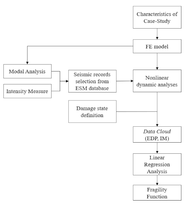
First, knowledge and choice of applications is paramount to obtain an FE model corresponding to the real system by taking into account all the possible uncertainties and weaknesses of the case-study system. A modal analysis needs to be performed, to describe the dynamic properties of the structure in terms of natural vibration period (T1), which is used to select a consistent range of intensity measure (IM). The number of selected records from European Strong Motion (ESM) database [53] needs to be established to ensure an appropriate distribution of cloud data. Then, the structure is subjected to a set of ground motion records by implementing nonlinear dynamic analyses. According to Limit State criteria and prescriptions by the reference seismic standards and guidelines, the value of Engineering Demand Parameter (EDP) for each ground motion record is employed to define the threshold with respect to which the fragility function has been constructed.

Within such a framework, linear regression analysis can be applied to cloud data to fit a lognormal curve for each EDP threshold, so as to derive the first two statistical moments (mean and standard deviation). Fragility curves finally represent the probability that the seismic response of the examined component exceeds an earthquake intensity parameter (IMi) conditional on the EDP threshold (EDPi) which is associated with a specific Limit State for glass. These data are presented in the form of cumulative distribution function as:

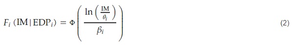
where:

• Φ denotes the standard normal cumulative distribution function;
• IM represents the intensity measure;
• EDPi corresponds to a specific value of demand parameter, which is representative of a damage state;
• θi is the median for IM given EDPi, which is derived from linear regression analysis as (a + b ln EDPi), where a and b represent the slope and intercept of linear fit, respectively;
• βi is the logarithmic standard deviation for IM given EDPi, which is calculated as square root of the estimate of the sampling variance by Equation (3):

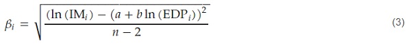
• n is the total number of samples, while i is the subscript representative of the damage state of interest.

3. Numerical Modelling of Case-Study Systems

The first example, CS#1, is a structural glass portal characterized by glass beam and columns with steel base joints. The second example, CS#2, is a sub-structure representative of a full-size glass wall bonded by a two-side adhesive layer. Such a system is considered as “non-structural” by most technical regulations, but can even affect the overall behaviour of the primary structure under seismic conditions. In both cases, the typical FE analysis consisted of two sub-steps, in which dead loads were first assigned to the system (quasi-static preliminary step) and the base horizontal acceleration was successively introduced to investigate the pre-loaded system (dynamic step).

3.1. CS#1: Structural Glass Frame

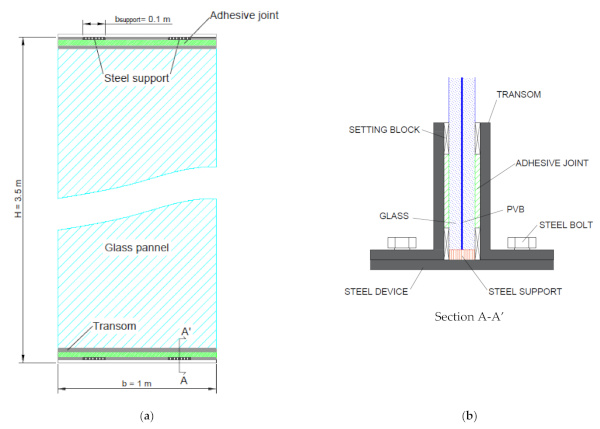
The system takes inspiration in geometrical and mechanical properties from the glass portal frame which was originally explored in [54] under in-plane seismic loads. As shown in Figure 2, the dimensions of the primary elements are 6 m for columns and 8 m for beams, respectively. The resisting cross-section of glass members has uniform size (600 × 66 mm) given by five glass layers (heat strengthened type, 12 mm in thickness) plus five interposed ionoplast foils (SG type, 1.52 mm in thickness).

The beam-to-column connection is characterized by an ideal pinned connection, while the base restraint of the frame consists of a bolted steel connection (M24 diameter), whose pins pass through two holes (32 mm its diameter) made in the laminated glass column, with a relative distance of D = 500 mm (Figure 1). Finally, four mild steel brackets fix the columns to the foundation. In terms of in-plane seismic response of the case-study system, critical issues are represented by the mechanical behaviour of base connections, where glass holes can be subjected to local stress peaks [54].

As a major variation from the investigation from [54], the current numerical analyses concerned an optimized modelling strategy that could facilitate the non-linear dynamic analysis of the whole frame, but also including the actual load-bearing mechanisms and damage of connection details. As such, the final FE model consisted of a combination of brick, shell and beam elements representative of glass frame components. Based on the nominal geometry in Figure 2, solid brick elements (C3D8R type) were used for steel angles, bolts and the interposed frictionless layers. A limited portion of glass column (0.6 m in height, thus corresponding to ≈1/10th the full column size) was described in detail, based on brick solid elements (in the region of holes) and shell elements (S4R type).

The shell-to-solid coupling constraint was used to merge the different portions of glass. Such a choice was privileged to have a good degree of accuracy for the analysis of stress peaks in the glass column, but at the same time to reduce the computational cost of parametric non-linear dynamic analyses. Regarding the resisting laminated section, for in-plane load purposes as in the present study, the viscous behaviour of interlayers was fully disregarded, and an equivalent monolithic glass member was taken into account for the column. Finally, a set of 1D rigid beams was used to describe the overall glazed frame in its elevation, so as to investigate the in-plane seismic response of the frame as a whole.

In doing so, the mesh pattern and size was optimized for separate regions and components of the FE model. The edge size for glass mesh was defined in the range from a minimum of 12 mm (holes region) up to 40 mm (top plate region). The final FE assembly resulted in 8600 solid/shell elements and 36,400 Degrees of Freedom (DOFs). An additional set of unsymmetrical non-linear surface contacts was included in FE simulations, so as to reproduce the actual mechanical behaviour of base device and its interaction with the region of glass holes [54]. This assumption facilitated the description of possible separation of joint components in tension and the reciprocal transmission of reaction forces in compression.

Finally, the mechanical properties for glass and steel were characterized based on nominal product standards, thus resulting in Eg = 70 GPa and Es = 210 GPa elastic moduli, νg = 0.23 and νs = 0.3 the corresponding Poisson ratio values and ρg = 2500 kg/m3 and ρs = 7800 kg/m3 the nominal density, respectively. As in [54], careful attention was paid for any possible fracture or yielding mechanism of materials, with σtk,g = 70 MPa the characteristic tensile resistance of heat strengthened glass (σck,g = 300 MPa the conventional strength in compression) and σy,s = 235 MPa the yielding stress for steel. The “Concrete Damaged Plasticity” law was adapted for glass from [54], while an elastic-plastic behaviour was taken into account for steel.

3.2. CS#2: Two-Side Adhesively Restrained Glass Wall

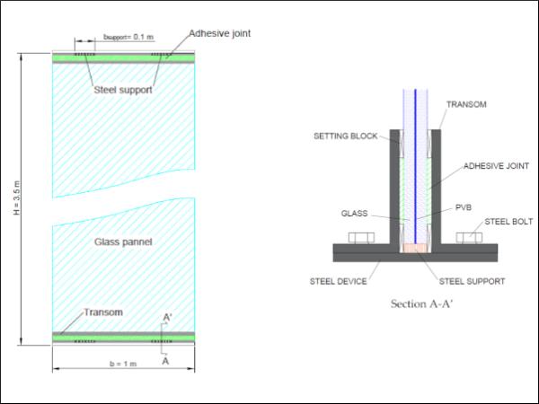
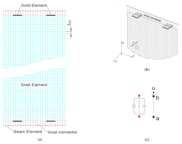
The second case study agrees with Figure 3 and represents a full-size glass wall, in which a single panel spanning between inter-storey floors (B × H = 1 × 3.5 m the nominal size) is characterized by the presence of two-side silicone restraints at the top/bottom edges. The nominal geometry of the examined system takes inspiration from [55,56], where the in-plane shear buckling response has been explored in detail. Generally, the use of this type of system is suggested to ensure lightness and transparency. On the other side, geometrical properties and restraints result in typically high flexibility, and thus potential vulnerability for these walls.

Literature studies are available to address the load-bearing capacity under in-plane loads and variable restraints [57,58,59]. In most of cases, the laminated (or insulated) glass panel is allocated inside metal restraints at the top/bottom edges, and rigidly connected to the structural background. No vertical members are used to provide additional stability and bracing to glass.

For the present study, the reference cross-section was assumed composed of two annealed glass plies (10 mm in thickness) and a middle Polyvinyl Butyral interlayer (PVB® type, 0.76 mm in thickness). Transoms for restraints consisted of two steel angles to avoid out-of-plane displacements along the top and bottom edges of glass, but at the same time to preserve the capacity of local in-plane sliding. A key role was thus assigned to the interposed sealant connection, and to a set of local setting blocks to preserve the compressive response of the system [55,56].

In order to predict the seismic behaviour of the examined panel, the reference FE model consisted of a combination of brick elements (C3D83 type) for restraints and shell elements (S4R type) for glass (Figure 4). Given the expected in-plane and out-of-plane deformations of the panel, a multilayer composite shell section was used to characterize the laminated glass wall in terms of bending stiffness parameters. For glass, the mechanical properties were described as for CS#1. In case of PVB film, for the assigned seismic action, the material behaviour was described in the form of equivalent secant stiffness for short-term duration load (30 s, see also [19]). Finally, the adhesive layers were described with a set of equally spaced axial connectors, so as to allow in-plane displacements (ux and uy) for the glass panel.

To this aim, the in-plane stiffness (Kx and Ky) per unit-of-length of each connector was calculated as for a commercial structural adhesive (Eadh = 2.4 MPa). The out-of-plane stiffness was set as infinite, thus reproducing the restraining effect of steel angles at the top/bottom edges of glass. Differing from CS#1, based on the regular features of the examined system, a regular mesh pattern was used for glass and supports. To preserve the accuracy of estimates and the computational efficiency of FE parametric analyses, the edge size for shell elements representative of laminated glass was set in 25 mm. The final result consisted in a total of 5800 elements and 36,000 DOFs.

3.3. Ground Motion and Intensity Measure (IM)

As a general rule, ground shaking due to seismic events is necessarily expressed as the simultaneous action of two horizontal components and a vertical one, which should be properly defined and even combined for structural analysis, depending on the structural typology object of study [27,28].

In case of (vertical) glass components with load-bearing capacity or even “secondary” role in buildings, design strategies are primarily focused on the in-plane and out-of-plane bending effects of horizontal components [32]. Such a general approach takes the form of simplified calculation methods as in Section 4, in which a local analysis is recommended for in-plane actions, in terms of glass and fixing systems. More specifically, the inter-storey drift (IDR) amplitudes caused by seismic actions are the first essential parameters for the design of glass members, but also for the optimal sizing of joints and connection systems, with respect to the characteristics of the rest of the structure/building assembly [32].

This is in line with classical setup arrangements for literature experimental studies on curtain wall components, and even numerical investigation for vertical glass members [25,60,61,62]. When possible, however, more complex setup configurations should be necessarily taken into account even for vertical load-bearing elements [63]. The vertical ground components should be definitely included for horizontal glass members (like slabs, roofs, or walkways that are sensitive to vertical vibrations [64]), in the same way of other constructional systems [65,66,67].

In the present study, based on selected standards and technical documents, as well as on the features of case-study systems, the attention was thus focused on the effects of in-plane lateral loads only, because of primary impact on the definition of the required EDP values. Further extension of the present investigation, in this regard, may also address the effects of spatial/three-axis earthquake records, as well as the structural interaction of glass components with the rest of building.

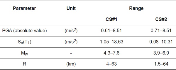
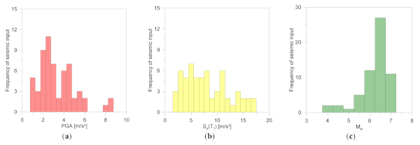
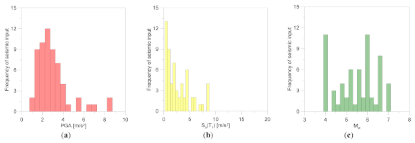
More in detail, a set of unscaled ground-motion records was considered to investigate the record-to-record variability of structural responses. Two different variables representative of the input seismic intensity were taken into account for the analysis of structural behaviours, namely the peak ground acceleration (PGA), and the spectral acceleration (Sa(T1)) corresponding to the fundamental period of each system (T1). Given that by generating a sufficiently large sample of events it is generally possible to minimize intrinsic randomness errors to “quite small” or “negligible”, the Cloud Analysis was carried out by considering a set of 60 unscaled accelerograms from the ESM database [53], for both CS#1 and CS#2. Table 1 shows the range of seismic events in use.

In addition to intensity measures (PGA and Sa(T1)), the parameters of moment magnitude (Mw) and epicentral distance (R) are reported, since representative of relevant seismic outputs to consider for quantitative measure of earthquake effects. According to EC8 classification [27], to minimize the influence of local effects, soil classes A and B were taken into account, thus corresponding to rock and very dense sand or very stiff clay soils, respectively.

Table 1. Characteristics of selected seismic events.

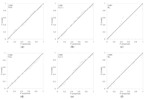
The final variation of input characteristics for seismic records is summarized in Figure 5 and Figure 6. It can be noted that the frequency histogram shapes typically recall a lognormal distribution, which generally is the most appropriate model to represent a seismic data set, as also reported in [68]. Figure 7 further confirms the global trend of examined parameters, and thus the appropriate selection of input signals [68], as it can be seen in terms of P-P plots for their lognormal distribution.

4. Definition of Performance Variables (EDP)

The first critical step to define fragility curves with the herein adopted analytical method is to identify the performance variables for the examined structural systems, and thus to establish damage thresholds. For glass structures, such a step may involve major uncertainties for design proposals, given that typical damage and failure mechanisms are affected by unsymmetrical (and brittle in tension) behaviour of glass or special restraint systems [19,54].

4.1. CS#1

For CS#1, the maximum IDR was chosen as reference EDP of the frame. Two different thresholds were derived with the support of push-over analysis of the system, with basic considerations about the expected collapse mechanism (i.e., glass fracture, steel yielding, etc.), as well as on the influence of the base connection on the overall seismic response (Figure 8). Given that the preliminary analysis of the framed system resulted in a primary collapse governed by glass cracking (in the region of bottom holes), but also characterized by the high flexibility and deformation capacity of the frame due to base joints [54], the attention of the present Cloud Analysis was focused on two different collapse conditions, namely detected as:

• Collapse “A”: corresponding to glass failure (tensile stress peak) for the column without base connection (i.e., rigid clamp at the base of the frame);
• Collapse “B”: referred to the whole frame system (tensile stress peak in the region of glass holes).

Such an assumption was quantified, respectively, in:

• (A) EDP = 0.048 m;
• (B) EDP = 0.35 m, corresponding to first glass cracking in the region of holes.

and thus enforcing the contribution of base restraints.

4.2. CS#2

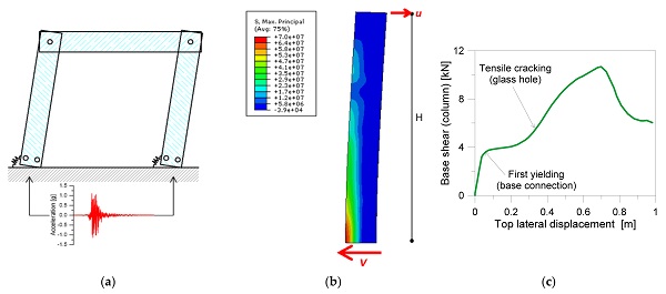
In terms of in-plane shear response, the CS#2 system is typically characterized by combined in-plane and out-of-pane deformations due to lack of vertical bracing systems and high flexibility of the laminated panel [56]. An example of stress distribution (both tensile and compressive) in glass, as well as the corresponding deformation and reaction force in the compression side can be observed in Figure 9.

For the fragility assessment of CS#2, further complexity in the present calculation process was found to derive from lack of technical knowledge about reference performance indicators for storefront configurations. In the field of structural engineering, existing regulations like the EC8 [27] or the Italian NTC2018 [28] classify glass components as “non-structural elements”. They are thus required to accommodate the relative seismic displacement (Dp) of the primary structure for a given Limit State of interest. However, a lack of analytical formulations able to predict the drift capacity of glazed systems has been recognized by several literature studies.

Moreover, it is reported in Section 4.3.5 that “Non-structural elements (appendages) of buildings (e.g., parapets, gables, antennae, mechanical appendages and equipment, curtain walls, partitions, railings, etc.) that might, in case of failure, cause risks to persons or affect the main structure of the building or services of critical facilities, shall, together with their supports, be verified to resist the design seismic action”. Similar recommendations can be found in the Italian CNR-DT 210 technical document for structural glass [32], where even non-structural members are required to absorb the deformations of the primary structure under the design seismic action, while maintaining their original load-bearing capacity towards vertical loads. Connections and restraints should be also properly verified.

According to [27,28,32], the effects of this seismic action on non-structural elements can be determined based on a simplified local analysis:

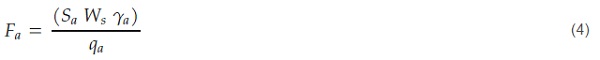
where:

• Fa is the horizontal seismic action applied in the centre of mass of the non-structural element, in the most unfavourable direction;
• Wa is the weight of the element;
• Sa is a seismic coefficient;
• γa is the importance factor, with a maximum value of 1;
• qa is the behaviour factor of the element (qa = 2 for facades, based on [27], but often sensitive to system details as discussed in [54]).

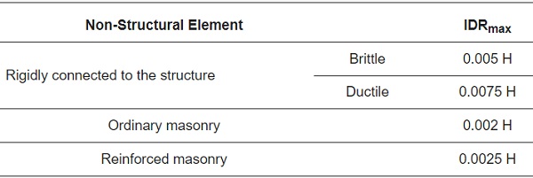
In addition to checks against local seismic actions (Equation (4)), the facade element is also required to accommodate the required Dp for a selected Limit State. A simple standardization of such a design requirement takes the form, as known for non-structural elements in general, from the preservation of possible damage due to a seismic action characterized by a greater probability of occurrence (“no-collapse requirement”) based on the limitation of relative deformations of floors. Typical reference values are reported in Table 2 and Table 3, in the form of maximum allowable inter-storey drift ratio (IDRmax).

Table 2. Reference limitations based on EC8 [27].

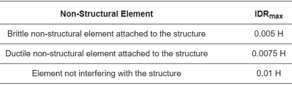
Table 3. Reference limitations based on NTC2018 [28].

A rational and practical definition of suitable EDPs and limit values should be taken into account also for glass, once the material properties and actual restraint mechanisms and capacities are taken into account.

In the present study, the in-plane horizontal relative displacement limit (Δfallout) was calculated as the maximum inter-storey displacement that the two-side adhesively restrained glass wall could accommodate without suffering for damage (“glass fallout”). Accordingly, the IDRmax threshold was calculated based on the reference value given by ASCE 7-10 document [29]:

ASCE 7-10 [29] also provides a formulation (Equation (6)) which can replace (when possible) a cyclic racking experimental test [30], to address the drift capacity of the glazing systems, or even detailed FE numerical analyses. The prerequisite is that the drift which causes contact between the glass panels and the bracing frame (Δclear) is:

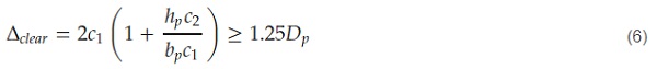
where:

• c1 = c2 = c is the average distance between glass panel and the surrounding frame;
• hp and bp represent the nominal size of the glass panel.

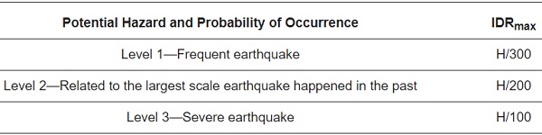
Finally, the Japanese code (JASS14) [31] specifies a maximum value of drift capacity of a given facade element in relation to the inter-storey height H, the severity of the seismic event and the probability of occurrence of the seismic event. Typical values are reported in Table 4. As shown, in the most serious condition of “severe earthquake”, the facade must be designed to satisfy a relative displacement up to 1% the inter-storey height.

Table 4. Reference limitations based on JASS14 [31].

Regarding the limitation of maximum out-of-plane deformations for the glass wall, the attention was set on the recommended limit values from the CNR-DT 210 document [32]. For a single glass panel in out-of-plane bending with 2-restrained edges, the maximum deformation in the transversal direction should not exceed:

where Linf corresponds to the height/bending span of the element to verify, depending on the spacing of restraints.

5. Discussion of Results

As also highlighted in Section 4, the present study aims at assessing the seismic performance of various glass system using a PBD approach, with a major intrinsic limitation that is characterized by weakness in definition of damage state thresholds. Generally, for a predetermined structure it is possible to accurately predict the level of ground acceleration that induces a certain level of response and/or state of damage. In addition to the characteristics of materials and other primary properties for seismic analyses (such as geometry, distribution of masses, stiffnesses), it is necessary to have information on the nature of site on which the structure is located. Obviously, it is not possible to have an exact deterministic knowledge of such information on the structure nor on the soil and on the seismic action, therefore it is necessary to make assumptions about the uncertainty with which such data are assumed.

5.1. Analysis of Sample Size (CS#1)

In order to address the sensitivity of fragility results, the influence of sample size generated on the statistical regression analyses for the examined CS#1 was investigated. To assess possible uncertainties in the adopted analysis method, the effect of number of samples on the estimation of parameters θ and β for Equation (2)—and determined by the mean least squares method—was analysed.

A repeated generation of statistical samples was carried out in groups of different size values. More precisely, the sources of considered randomness took the form of (i) magnitude of dead vertical load on each column (P0) and (ii) Young’s modulus of glass (Eg). Both these two entities were considered as discrete random variables with a constant probability density, by means of three values which explored the field of interest (Table 5). Regarding the tensile and compressive resistance of glass, no variation was taken into account from nominal parameters, given that the imposed seismic records generally resulted in stress peaks in in the order of ≈1/4th the characteristic material strength (elastic response). Such a set of assumptions resulted in the generation of a statistical sample in which a total of 540 non-linear analyses were carried out, by combining seismic input variability with the structural uncertainties summarized in Table 5.

Table 5. Considered values for input variables in CS#1, in terms of Young’s modulus of glass (Eg) and dead vertical load (P0).

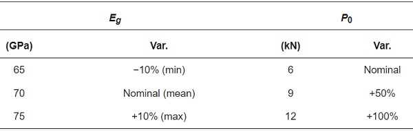
Regarding the Eg values in Table 5, in accordance with [69], the reference interval was calculated as:

with:

the standard deviation.

In terms of vertical dead load P0, it has to be noted that initial value P0 = 6 kN representative of sustained frame members and conventional accidental load was calculated to correspond to limited compressive stress ratio for the glass column, that is:

where Ag = 36,000 mm2 represents the cross-sectional surface of glass layers only. For this reason, the numerical analysis was carried out by increasing up to +100% the so assigned load (Table 5). The collected fragility parameters as in Equation (2) were thus addressed for the 60 or 540 samples, respectively.

Figure 10 and Figure 11 show the difference between linear fits in terms of R-squared, a statistical measure of how close data are to the fitted regression line, which can be computed as:

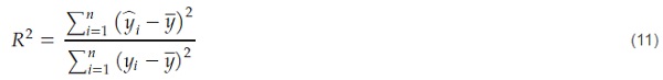
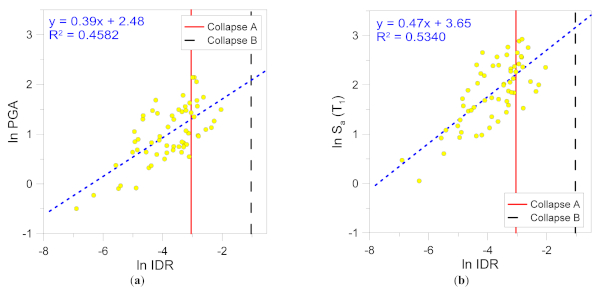
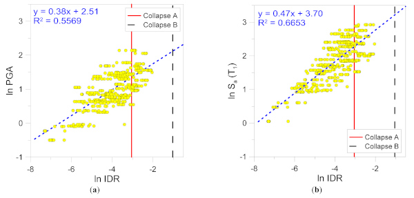
In Equation (11), 𝑦̂𝑖 are the estimated data from the model (with i = 1, ..., n), 𝑦𝑖 are the experimentally observed data and 𝑦̲¯ their average value. The term to the numerator has therefore the meaning of deviation explained by the model, while the denominator represents the total variance of the examined population. The higher the R-squared, the better the model fits data cloud.

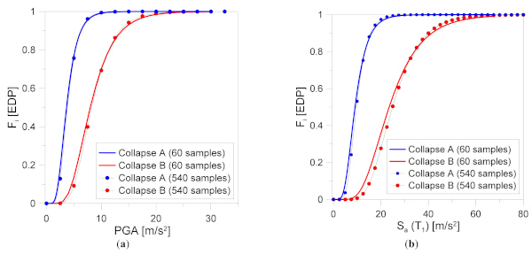
Numerical results are proposed in Figure 10 and Figure 11 both as a function of PGA and Sa(T1). The effect of sample size can be noticed by comparison of charts. In particular, the confidence band is represented by the limits of plus/minus one or two standard deviations from the median, which corresponds to approximately ≈70% and ≈95% probability, respectively, based on normal distribution [68,70]. As shown, a monotonically decreasing trend with respect to the number of employed records can be observed.

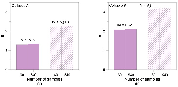
Finally, the variation of the first two statistical moments θ and β from Equation (2) is shown in Figure 12 and Figure 13, respectively. As it can be noticed in Figure 12, the sample size results in a θ variation up to ≈3.5% (Collapse A) or ≈1.6% (Collapse B) for PGA intensity measure. Such a scatter in θ reduces to ≈2.8% (Collapse A) or ≈1.6% (Collapse B) for Sa(T1). The increase of θ from Collapse A to B is calculated in the order of ≈30%, both in terms of PGA or Sa(T1).

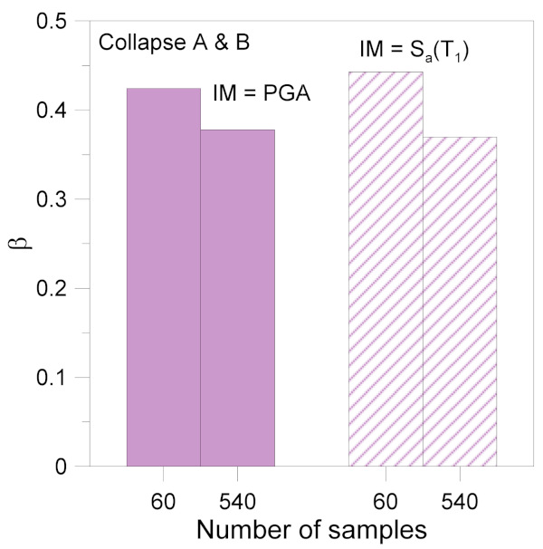
The analysis of β trends in Figure 13 shows that the sample size results in a scatter up to ≈19% in terms of PGA and ≈13% in terms of Sa(T1). It has to be noted, moreover, that β does not depend on the given collapse mechanism (A or B), thanks to basic heteroscedasticity hypothesis.

5.2. Analysis of EDP Thresolds (CS#2)

Dealing with CS#2, several literature studies highlighted that the response of a full-size glass panel can be often described in two steps for a fully framed pane:

• Following the deformation of the frame, the glass panel firstly moves in the direction of the seismic action until contact is generated between the frame and the sheet with subsequent rotation of the glass panel itself;
• The glass panel is then stressed at opposite corners by a compressive load deriving from the deformation of the frame/bracings. In this phase, the glass element tends to bend and at the same time to shorten along the diagonal with consequent out-of-plane deformations that should be properly verified.

Consequently, both the in-plane and out-of-plane performance of CS#2 was investigated under seismic action. In the former case, glass fallout was considered as primary damage state due to the imposed earthquakes events. Such an ultimate Limit State occurs at a particular value of drift, which should be derived from experimental tests or regulatory instructions. In the present study, comparative FE estimates from numerical analyses are addressed towards reference limits summarized in Section 4. 

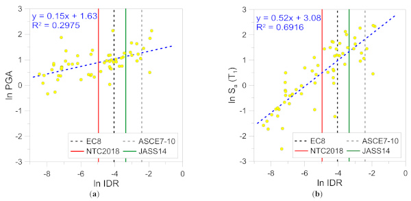
Figure 14 shows major outcomes from numerical analyses (data clouds), linear fits and the chosen IDR thresholds by which the probabilistic parameters θ and β are derived. Worth to note, depending on the used technical document, the high sensitivity and variability of limit IDRmax parameters for a given glass system to verify. As an additional aspect to point out, the parametric FE simulations as in Figure 14 typically resulted in stress peaks in glass (i.e., middle region in bending and detail of supports as in Figure 9) typically lower than the reference strength parameters (elastic stage), both in tension and compression.

6. Derivation of Fragility Curves (CS#1 and CS#2)

At a final stage, fragility functions were evaluated for both CS#1 and CS#2 systems in terms of EDP thresholds corresponding to specific drift limits for each case study, as also discussed in Section 4. Both PGA and Sa(T1) values were used as alternative intensity measures on the x-axis of fragility functions.

Major outcomes are proposed in Figure 15, Figure 16 and Figure 17 for CS#1 and CS#2, respectively. In both cases, it is possible to notice that the use of a reference drift value as a function of the limit condition of interest (which can be derived from refined structural analysis, as for CS#1, or from literature design standards, as for CS#2), as well as the selection method to derive seismic inputs have both a significant effect on the resulting estimates of expected structural response. Such an effect is particularly evident when design Sa(T1) is used as intensity measure.

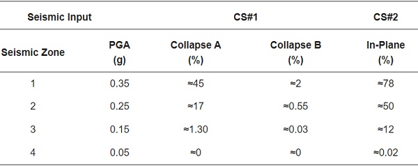
In particular, it is possible to notice in Figure 15 that the frame analysis (CS#1) inclusive or not of mechanical and loading uncertainties leads to an error of approximately ≈10% for Collapse A and ≈6% for Collapse B, respectively, corresponding to the lowest value of IM with a unit probability. To better understand the seismic performance of the system and compare it to existing design recommendations, it is also useful to discuss numerical results in terms seismicity levels and associated PGA ranges. The presently used PGA values correspond in fact to the Italian scenario (Table 6), namely to four zones representative of different hazard levels. For example, for seismic zone 1 associated with very high seismicity (PGA = 0.35 g = 3.43 m/s2), the expected probability of CS#1 for Collapse A is about ≈45%, but less than ≈2% for Collapse B. The collected results prove consequently that a very low seismic damage can be expected even for high intensity measure.

Table 6. Reference seismic zones and anchorage acceleration of the elastic response spectrum (PGA), based on OPCM3274 [71] and approximate expected collapse/damage probability for CS#1 and CS#2.

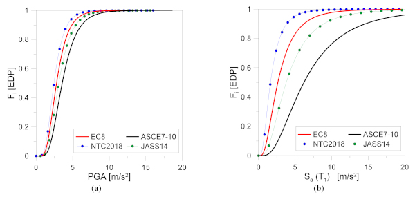
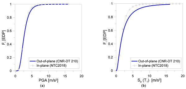
For CS#2, fragility functions are proposed in Figure 16 and Figure 17, with attention for in-plane and out-of-plane displacements, respectively. The comparative analysis is based on different threshold limits as from the selected design standards discussed in Section 4. In case of out-of-plane deformations, the reference limit value is taken as in Equation (7).

More in detail, see Table 6, the analyses clearly point out the largest vulnerability of the system respect to the glass frame in CS#1 and, consequently, a significant probability of damage corresponding to the same intensity of earthquake event. In fact, in case of fragility function for in-plane performance with a PGA equal to 3.43 m/s2 (i.e., seismic zone 1 from Table 6), the maximum value of expected probability of exceedance is about ≈78%, which is almost double compared to the calculated value for CS#1.

Worth to be noted that for upper bound (PGA = 0.25 g = 2.45 m/s2) and lower bound (PGA = 0.15 g = 1.47 m/s2) of medium seismicity range (being the most common cases in Europe), the probability of exceedance at the site of interest is about ≈50% and ≈12%, respectively for CS#2, thus still more pronounced than CS#1 (Table 6).

Finally, as shown in Figure 16, the performance indicators provided by NTC2018 standard result in a most severe fragility function for the examined system, while the ASCE7-10 limit condition can be associated with less conservative predictions. Such an outcome is particularly emphasized for fragility curves in terms of Sa(T1). For fragility estimates in terms of PGA, a less pronounced scatter can be noticed from Figure 16a. The probability of collapse for seismic zone 1, for example, is in the order of ≈78% based on NTC2018, but up to ≈45% for ASCE7-10 limit parameters.

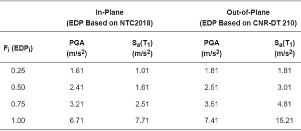
By comparing the in-plane and out-of-plane performance of CS#2 as reported in Figure 16 and Figure 17, it is also possible to address the reliability and severity of selected performance indicators for the examined system. Such a step can be carried out by means of a quantitative comparison of selected values of cumulative function Fi.

To this aim, Figure 17 reports the in-plane fragility function based on NTC2018, for graphical match with the out-of-plane indicators. Quantitative comparisons are further summarized in Table 7. The selected data, as shown, prove that the in-plane lateral displacement represents, both for PGA and Sa(T1), the most severe condition in case of seismic analysis for facade components. Such an outcome confirms the accuracy of simplified design procedures as discussed in Section 4. At the same time, the comparative analysis gives evidence of rather close correlation for in-plane and out-of-plane fragility functions as in Figure 17a, thus suggesting a further dedicated analysis of performance indicators for generalized proposals.

Table 7. Comparative analysis of in-plane and out-of-plane variables for selected values of fragility functions (CS#2).

7. Conclusions

An increasingly popular method to probabilistically characterize the seismic response of a given structure is based on the use of “fragility” or “seismic vulnerability” curves. Most of existing applications, however, typically refer to constructions and structural members composed of traditional building materials.

The present study intended to lay the basis to obtain fragility analysis results as necessary tools for a performance-based design (PBD) process. The attention was focused on the fragility assessment of glass structures and components in buildings, based on two different case-study systems (i.e., a glass portal frame, CS#1, and a two-side adhesively restrained glass wall, CS#2). A major advantage was taken from by the use of Cloud Analysis in the Cornell’s reliability method, and its adaptation for the seismic assessment of glass building components, and refined Finite Element (FE) numerical models for non-linear dynamic simulations.

The analysis of structural reliability, as known, depends on the level of knowledge of random variables, but also on the type of required assessment. The basic issue in dealing with glass material, in general, is the lack of specific regulations and studies on the probability function that can be used to represent material and structure uncertainties in a sampling method (i.e., Monte Carlo or Latin Hypercube Sampling). Based on the findings discussed in the paper, it was proved that the evaluation of structural reliability of a glass system in seismic region cannot be generally addressed with a simple deterministic approach. The problem indeed necessarily requires to take into account the statistical variability of input parameters. For the present study, another major source of uncertainty in the assessment of structural behaviour of glass components was found in the randomness of seismic actions.

From the non-linear dynamic analysis of selected glass structures, as well as from the development of proposed fragility curves, the presented results proved that:

• In order to assess the reliability and structural integrity of glass building components, the Cloud Method can be used to address their behaviour under seismic actions. As shown, however, the method itself may be affected by uncertainties related to material properties, number of parameters involved, sample size, and reference Engineering Demand Parameters (EDPs);
• The development and fine-tuning of a numerical model should properly consider different components (glass, restraints, gaskets, etc.), as well as their mechanical interactions under in-plane and out-of-plane deformations. Numerical simplifications (especially in boundaries) may result in non-accurate seismic analyses, and thus inappropriate predictions for the definition of coherent drift capacities;
• Often, due to restraint devices or bracing systems that are typical of structural glass applications, very high flexibility, and deformation capacity can be observed before any damage mechanism occurs in glass (or other structural components). Reliable performance indicators, as shown, should be thus considered for specific boundary conditions;
• Based on glass material properties, fragility analyses may be severely affected by the unsymmetrical behaviour of material itself, with limited tensile resistance in tension compared to the compressive capacity. Especially in presence of holes, bespoke restraints, etc., such a mechanical behaviour needs specific constitutive laws and damage mechanisms to be included;
• In conclusion: the present study confirmed the potential of fragility curves for different glass systems in buildings. However, further verification of procedural steps is required towards the definition of generalized EDP values for categories of structural typologies/boundaries. Such a goal will be addressed with more case studies, different number of earthquake records and a probabilistic treatment of the involved uncertainties.

Author Contributions

All authors have read and agreed to the current version of the manuscript. Conceptualization, S.M. and C.B.; methodology, S.M. and C.B.; investigation, S.M. and C.B.; supervision, C.B. Both authors have read and agreed to the published version of the manuscript.

Funding

This research received no external funding.

Informed Consent Statement

Not available.

Data Availability Statement

Supporting data will be made available upon request.

Conflicts of Interest

The authors declare no conflict of interest.

References