Investigation of cooling systems in a glass grinding process

This paper was first presented at GPD 2023.

Link to the full GPD 2023 conference book: https://www.gpd.fi/GPD2023_proceedings_book/

Authors:

Adrian Lareida, Fikri Mert Ilten, Michal Kuffa and Konrad Wegener

Abstract 

Edge grinding is an important process step in the manufacturing of glass for automobile and display industry. Short cycle times demand high material removal rates of the grinding wheel. Coolant needs to be supplied to achieve a time wise efficient grinding process without melting the glass.

Different cooling systems are tested against a standard coolant system in a series of experiments. Their performance in terms of edge surface roughness and grinding wheel wear is being compared.

Intensive studies for all cooling systems involving laser profiling and 3D microscopy for wear analysis are performed. Attritious wheel wear is detected indirectly due to grinding current increase.

Furthermore, it is found that a single nozzle directed towards the contact zone is sufficient to cool the process, which reduces the amount of coolant necessary by a factor of up to 10. A force model is tested, which is implemented in a kinematic geometric grinding simulation tool. The force model is the base for further models for temperature and wear, which can be implemented as well.

Introduction

The process of glass grinding

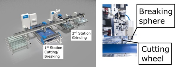
On a system for glass processing such as that offered by Glaston, for example, the glass is separated in four process steps. The glass is delivered in mostly rectangular raw shapes and brought by suction cups to the first station. At the first station, shown in Figure 1 on the left, the glass surface is scored by means of a cutting wheel. The scribing of the glass shapes the contour of the final product.

In the next step, the glass is broken at the same station. The cracks that were added during the cutting ensure that the glass breaks in the desired places. The breaking itself is done with a so-called breaking sphere, which is moved on the surface under a set pressure. The arrangement of the cutting wheel and the breaking ball is shown in Figure 1 on the right. The shape cut and crushed from the raw form is then transferred to the next station. At the second station, the glass edge is ground. The glass is sucked up by vacuum cups on a rotating table. The grinding wheel moves to the edge of the glass and grinds it off with the usual infeed of 0.3 mm. In the cases examined here, the grinding wheel has a concave C-profile.

The feed rate is generated by the rotation of the rotary table, which is in the range of 15 to 45 m/min. In most cases, one rotation is sufficient to achieve the desired quality. However, multiple grinding cycles can be programmed, including other grinding wheels, which can be selected by moving along the spindle axis. This completes the process on this line. The next step for most applications is to go through a washing system.

Coolant systems in the grinding field

Cooling in grinding is necessary in many cases. Often the shape of the abrasive grains causes a high heat emission during material removal. This heat must be removed from the machining zone. Grinding burn is a well-known phenomenon that occurs when cooling was insufficient. When grinding glass, one speaks of so-called "firing". Firing is visible by glowing sparks and an associated sharp increase in spindle current. The glass edge melts and the glass gets a characteristic white layer. For quality reasons, this must be avoided.

Reviews of cooling systems [1-2] show the classification according to the type of cooling medium. A distinction is made between liquid, gaseous and solid cooling media. The liquid media are further subdivided into oil-based and water-based coolants. For gaseous media, the focus is on cryogenic media such as liquid nitrogen or liquid carbon dioxide. The solid cooling media are graphite, molybdenum disulphide or titanium aluminium nitride. Oils can also be further divided into vegetable, animal, synthetic and mineral oils. Due to environmental compatibility, the use of vegetable instead of mineral oils is the subject of research.

Nanofluids are another category of liquid coolants. Here, nanometre-sized solid particles, for example carbon nanotubes, aluminium oxide, molybdenum disulphide, graphene or even diamond, are introduced into a liquid medium. These particles increase the heat capacity and at the same time reduce the friction between the tool and the workpiece. Due to these improved properties, the volume flow can be reduced.

For the supply of coolants, a distinction can be made between flood cooling and minimum quantity lubrication (MQL) depending on quantity. Because today's flood cooling systems account for a high proportion of production costs, as Sanchez et al. show in [3], switching to MQL is a goal in the industry. Using an example from the automotive industry, Sanchez et al. [3] estimated the cooling system cost to be two and a half times the tooling cost. More than 60 % of the cooling system costs are equipment costs (40 %) and waste disposal costs (22 %).

Kinematic-geometric simulation programme 

The ability to simulate a grinding process is a powerful and flexible tool for investigating the relationships between process parameters and their effect on the result. This allows the process to be understood in detail and optimal settings to be found. At the Institute of Machine Tools and Manufacturing at ETH Zurich, a dedicated simulation programme for abrasive processes is currently being developed. The processes are modelled using a kinematic geometric approach because this method offers the necessary precision and complexity required by abrasive processes, but at the same time requires less computing power than other complex methods such as molecular dynamics or the finite element method. The aim of the simulation programme is to predict and optimise abrasive processes in terms of surface quality, less tool wear, faster material removal, etc.

The simulation programme is written in the Python™ programming language, following an object-oriented programming approach. The reason for this approach is the resulting modular structure for the simulations. The basic possibilities, namely collisions and material removal, are implemented with as few assumptions as possible, so that a high range of processes can be simulated. By specifying the process kinematics, the tool and physical models for forces, wear and temperatures, users can set up their processes in the simulation programme. Tools can be created by predefined geometries or by importing meshes of the grains. Various standard models such as the Kienzle force model or the Usui wear model can be selected. In addition, own models can also be implemented. Several simulations with different parameters can be started from a single input file. Furthermore, the simulation programme offers several options for the evaluation of the simulation, for example, the material removal and forces on the tool or grit level, topographies of the tool and workpiece, average and accumulated wear, etc.

Material and Methods

Cooling systems structure 

Three different cooling systems were tested. Namely:

• Standard splash ring (SSR) 
• Optimised standard splash ring (OSR) 
• Tangential splash ring (TSR)

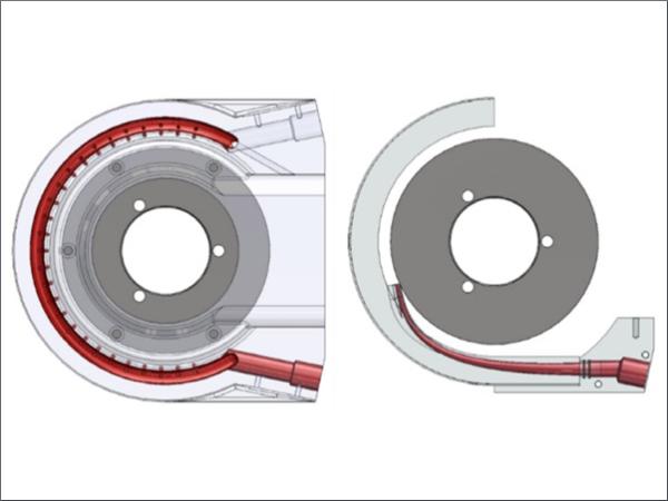
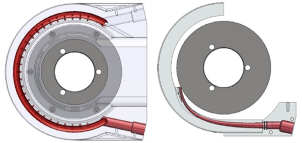
The SSR is shown in Figure 2. It has 27 nozzles evenly distributed around the grinding wheel. In comparison, the TSR has a single nozzle, which is pointed at the contact zone when machining circular discs. The OSR is very similar to the SSR, there are only minor changes, such as the number of nozzles, which has been slightly increased, and the angle of the nozzles, which has been adjusted.

The SSR and OSR are made of aluminium. In contrast, the TSR is made of polyamide and was not machined conventionally, but by means of selective laser sintering (SLS). The injection rings are connected to a coolant supply consisting of a coolant tank, pump and diaphragm valve for volume flow control. For the SSR, the usual volume flow is in the range of 30 to 90 l/min. The TSR consumes around 5.5 l/min.

Grinding wheel specification 

A metal-bonded diamond grinding wheel was used in the experiments. The diamond grains have an average grain diameter of 82.5 µm and a ratio of grain area to total area of 0.25. The wheel has a concave C-profile with a radius of 1.6 mm and is suitable for the glass thickness of 2.85 mm used. The outer grinding wheel diameter was 150 mm. The cutting speed was set at 50 m/s and the feed rate at 30 m/min.

Evaluations

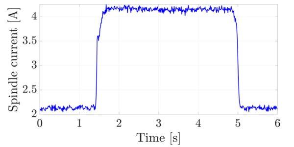
Current: The spindle current is already being recorded and was therefore also evaluated. The current value can also be converted to forces and power. The conversion takes into account the change in diameter after sharpening the grinding wheel. During regrinding, the first phase of the raw spindle current curve is the “idle” current consisting of spindle rotation and cooling water resistance, followed by an area where grinding takes place. Towards the end, the current consumption drops again and grinding is finished there. An example of such a curve is shown in Figure 3. For the analysis, the arithmetic mean of the constant areas was calculated. Both when looping and when determining the “idle” current. This gives one value per loop.

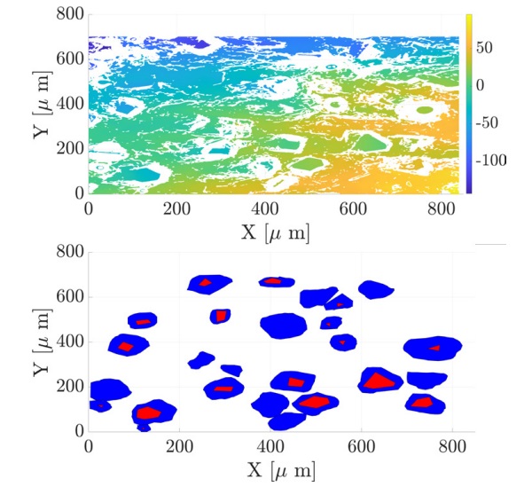
Grinding wheel profile: In order to record the profile of the grinding wheel at different times, imprints were made using imprint silicone Accutrans® from Coltene. These could then later be measured under the Sensofar S neox 3D microscope and their topology evaluated. The method was originally presented in the Doctoral Thesis by Wunder [4]. An example of the measurement is shown in Figure 4. The diamond grains were marked manually, from which evaluations were then made. The diamond area versus the total area was considered, the protrusion height as the maximum distance between the grain tips and the averaged plane of the embedding environment, and the diamond tip areas versus the embedded area.

In addition, the bearing surface curves were also calculated from the point clouds obtained. All lines in the X-direction and all lines in the Y-direction were used for this. Missing values were linearly interpolated and an overall curve could be arithmetically averaged from them. 

Furthermore, the system used has a 2D line laser from Micro-Epsilon. This is used as the standard to determine the diameter of the grinding wheel. The measurement is made by averaging the measured points while the grinding wheel is rotating. The profile can also be read. In addition, except for the experiments with the SSR at 30 l/min, measurements were made with an external 2D line laser, also from Micro-Epsilon. The grinding wheel was at a standstill and the profile obtained was evaluated in the same way as from the internal sensor. The differences in the profile depths of the individual measurements were chosen for evaluation.

Glass surface: The roughness profiles of the one-off and the fifty times reground glass sheets were recorded using the Taylor Hobson Form Talysurf Series 2 stylus instrument. The roughness and waviness profiles were determined according to ISO 4288 [5]. However, measurements were taken at right angles to the measuring direction specified in the standard and the measuring section length was also selected one category shorter. The values obtained are therefore only comparable among the individual samples, not with roughness and waviness values from other publications.

Coolant pressure: A Cerabar S pressure sensor from Endress und Hauser was mounted before the inlet to the splash ring. This enabled measurements of the coolant pressure. The pressure was measured to record any blockages in the nozzles. Because the pressure remained constant and no abnormalities were observed, an evaluation in the results and discussion chapter is omitted.

Experiments and Simulations

Experimental procedure 

Series 1: «Without glass»: A series of tests without glass was carried out with the SSR. The amount of coolant was reduced from 80 l/min to 0 l/min in steps of 20 l/min. The aim was to investigate the effect of the cooling water quantity on the spindle current.

Series 2: «Influence of sharpening and cooling water quantity»: To see how much the amount of coolant can be reduced, a series of tests was carried out with the SSR. In the process, a glass was first ground around ten times and then a dressing process was performed. This was done with the standard 60 l/min. Another two times were repeated to investigate the influence of the sharpening at the same time. Then the glass was ground another ten times at 80 l/min. The amount of coolant was then reduced to 40 l/min. At the next reduction to 20 l/min, firing was detected and the amount of cooling water was increased to 30 l/min. No further sharpening was done during these grinding sets.

Series 3: «Comparison of coolant systems»: The SSR was compared with the OSR and the TSR. With the SSR, two coolant quantities were tested, namely 60 l/min and 30 l/min. Thus, the test procedure was carried out four times. This consisted of the following steps:

• Sharpening of grinding wheel 
• Make an imprint of the fresh grinding wheel 
• Cut and break the first glass and grind around once
• Cut and break second glass and grind around 50 times
• Create “half-time” imprint
• Cut and break third glass and grind around once
• Cut and break the fourth glass and grind around 50 times
• Cut and break the fifth glass and grind around once
• Create imprint “before sharpening”

Simulations 

The simulations were carried out with the internally developed simulation programme described in the introduction.

Geometry: Grains were selected according to the size distributions in the experiments with a mean diameter of 82.5 µm and a standard deviation of 3 µm. The shape of the grains was randomly selected from cuboctahedra, slightly truncated and truncated octahedra. Different grain densities were simulated to find a correlation between the number of grains and process forces. Thus, later simulations can be carried out with reduced grain density, which greatly reduces the simulation time. The glass thickness was specified as 2.85 mm, as in the experiments.

Kinematics: The feed rate and speed were taken from the experiments and were 30 m/min and 6496 min⁻¹ respectively. The simulation was carried out on straight glass edges instead of round glass edges as in the experiments. This difference can be compensated by multiplying the current value by the voltage and dividing by the corresponding material removal rate.

Force model: The force model used in the simulation is based on the work of Jiang et al. [6]. The grains were categorised into different stages, the stages being "contactless", "sliding", "ploughing", "cutting". For the latter two stages, force models by Hecker et al. [7] and Merchant [8] were used. The classification into the different stages is done according to equation (1).

Here dgx is the grain diameter, ξcut is a grading factor of 0.025 and hcuz is the penetration depth of the grain. According to the article by Jiang et al. [6], the "sliding" of the grain can be neglected. Thus, a grain is either "contactless" when it does not penetrate the glass surface, "ploughing" when the actual penetration depth is smaller than the penetration depth from (1) and "cutting" in the other case.

The equations for the normal force Fn and tangential force Ft for the grains in the ploughing stage are therefore

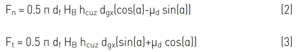
Here df is an empirical factor of 0.3, which includes the shape deviation of the grain from a sphere, the high cutting speeds and the change in material properties at high temperatures [7]. HB is the Brinell hardness of 438.5 MPa from [9] for soda-lime glass and µd is the coefficient of friction between the workpiece and the tool, which was assumed to be 0.1. The fact that the coefficient of friction can change with different cooling was neglected. The entry angle of the grain is denoted by α. For the grains in the cutting stage, the normal and tangential forces are described according to equation (4) and equation (5) respectively.

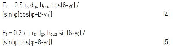
Where τs is the shear yield strength, for a first assumption equated with the yield strength of soda-lime glass at 32.5 MPa [9]. β is the friction angle of an intersecting grain, γ0 the rake angle of the grain, and φ the shear angle.

Wear model: Due to the short processing time during the experiments, the use of a wear model was omitted.

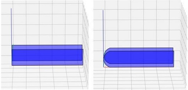
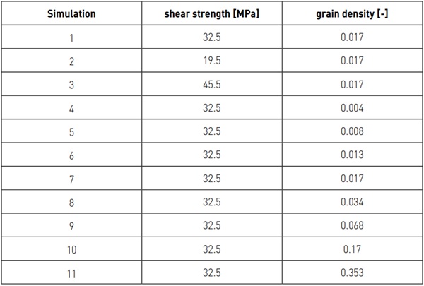
Design of Experiments: For the simulations, the shear strength and grain density parameters were varied. The shear strength was varied to ensure that this factor behaved linearly, as shown in equations (4) and (5). In a first iteration, the simulation settings in Table 1 were adopted. Later, the shear strength was adjusted according to the results obtained and tested by simulations on glasses that already had a C-profile. A representation of the simulated profiles is shown in Figure 5.

Simulations 10 and 11 were carried out with three different starting values for the randomness variables. This is to show that the grain size, grain orientation and grain position distribution have no influence on the result, namely the spindle current, due to the high number of grains.

The conversion from torque to spindle current was done with equation (6).

Here I is the current, T the torque, U the voltage (375 V) and ω the angular velocity.

Results and discussion

Series 1: «Without glass» 

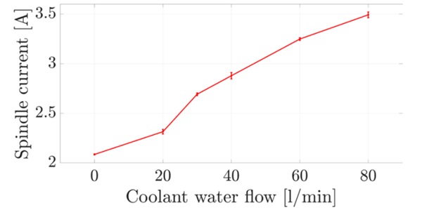
The averaged current values for the selected coolant quantities are shown in Figure 6. As can be seen, the current value without coolant, i.e. only with spindle rotation, is 2.08 A. Above 30 l/min, the increase in current consumption is almost linear to the increase in coolant. At 20 l/min the current consumption is lower, with the reasoning that due to the low impulse of the "slow" water, a large part is sucked upwards and therefore there is no resistance for the spindle.

Series 2: «Influence of sharpening and cooling water quantity»

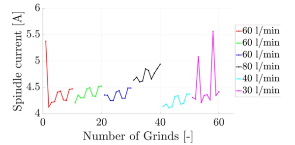
Figure 7 shows the average spindle current values compared to the individual grindings of the test glasses. At the beginning, the glass edge was still right-angled, which is where the increased current value comes from. As soon as the glass edge has a C-profile shape, the current consumption decreases because less material has to be ground away. The two peaks towards the end at 30 l/min can be explained by the fact that firing occurred briefly during these regrinds because the cooling water did not reach the grinding zone. The same reasoning with the low impulse of the water as described in 4.1 applies here. The alternating zigzag behaviour of the current values is based on the programming of the CNC control. When using multiple looping, the control changes. The difference between the controls lies in the maximum acceleration. Therefore, the current value is lower with the slow control with a maximum acceleration of 0.7 m/s2. If we compare the first 30 regrinds, which were carried out with 60 l/min, we can see that sharpening resets the current consumption after every 10 regrinds.

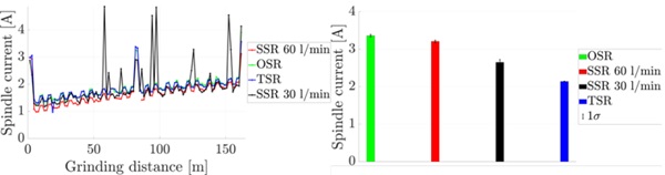
Series 3: «Comparison coolant systems» 

The spindle power consumption compared to the ground metres is shown in Figure 8. The peaks at the beginning, at the halfway point and at the end are due to the already mentioned right-angled glass edge in the newly broken glasses. The peaks at the SSR with 30 l/min in between can be explained by firing. Basically, it can be seen that the net power consumption is the same for all systems. This means that no system has an improved lubricating effect. It can also be seen that the power consumption increases continuously compared to the grinding path. With the SSR with 60 l/min, the power consumption increases faster than with the other systems. 

A possible explanation would be that the first tests were carried out with this spray ring and any external influences such as machine expansion played a role. The reason for the general increase in current is probably the wear of the diamonds. The power consumption due to spindle rotation and the resistance applied by the coolant is significant. Figure 8 on the right shows the spindle currents with the cooling systems switched on. The OSR has the highest current consumption, followed by the SSR with 60 l/ min and then with 30 l/min. Only 0.05 A more than idle is required by the TSR. The increase in current due to this solution is thus negligible. However, the tangential injection does not provide a positive effect either, so the system does not work according to a "waterwheel principle". This can be explained by the higher circumferential speed of the grinding wheel compared to the water jet speed.

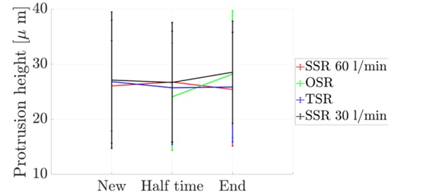
No differences over time were observed when viewing the grinding wheel profiles using the imprints under the microscope. Figure 9 shows the protrusion height of the individual splash rings. The corresponding standard deviation applies to the distribution of the individual protrusion heights. On average, the protrusion height is about 27 µm, i.e. about one third of the grain diameter.

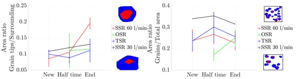
The area ratios of grain tips to embedding surrounds, as well as the area ratios of grain area to total area, are shown in Figure 10. The area ratio of the grain tips increases slightly, indicating wear of the diamonds. Why the increase is so strong for the SSR cannot be explained. The area ratio of grains increases up to the halfway point for the SSR and TSR, and then drops again. For the OSR, only data from half-time to the end are available. The opposite behaviour is observed there.

In order to determine greater effects, grinding would have to be carried out over a greater distance in the kilometre range. The increase in current can be explained by micro-wear of the diamond grains. The micro-wear cannot be measured by the evaluations; blunting of the diamond grit must be investigated in more detail. An increase in current due to grinding dust settling on the grinding wheel is unlikely, as the increase was approximately the same for all splash rings, although the cleaning effect should be different. The grinding wheel is also hardly porous, so the settling of grinding dust is not promoted.

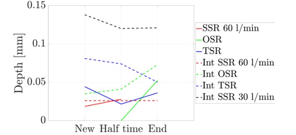
The comparison of the relative profile depths with the measurements of the laser sensors also shows hardly any changes. Figure 11 shows the profile depths. The test with the SSR at 30 l/min was carried out later than the others, which is why the relative profile depth is highest there. The changes in the profile depth are in the 10-1 mm range, the wear of the grinding wheel therefore minimal. Measuring the glass surfaces with the stylus instrument revealed periodic waviness. An example profile is shown in Figure 12. 

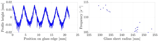
In order to analyse the wave frequency more precisely, the signal periodicity was therefore determined by means of autocorrelation. The frequencies obtained were examined in more detail. To convert periodicity length lp into a frequency f, the respective feed rate vf was chosen. The corresponding equation is given in (7).

It is shown that the frequencies are dependent on the total radius of the glass pane. The frequencies correlate negatively with the radius of the glass pane. The correlation is shown in Figure 12 on the right. At a spindle frequency of 108 s⁻¹, the trigger for this waviness is also found.

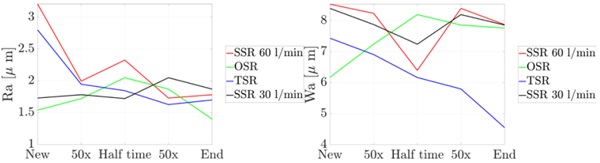
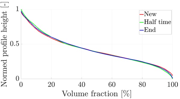
The values for roughness (Ra) and waviness (Wa) were also calculated and are shown in Figure 13 on the left and right, respectively. The TSR convinces with low roughness values. Both the TSR and the SSR with 60 l/min required a "running-in" period at the beginning after sharpening. After that, the roughness and waviness values are constant or decreasing. For the SSR with 30 l/min, Figure 14 shows the normalised bearing surface curve (AbbottFirestone curve) at the different measuring times. Practically no change can be detected over the experiment time. This supports the argument that at most a difference in grain sharpness occurred.

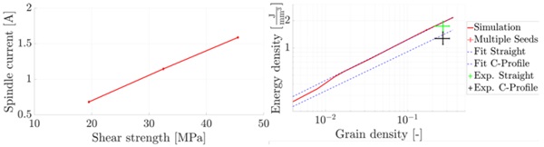
A power law is suitable for fitting, since the current increase in the corresponding double-logarithmic plot is linear. The value of the multiplier is 3.452 and the value of the exponent is 0.448. To bring the simulations into agreement with the experiments, the shear strength must be reduced to 29.54 MPa. This value was tested on the second geometry, which was ground. This geometry consisted of an already C-profile edge. The mean values from the first experiments when grinding the C-profile were taken and two simulations with grain densities of 0.017 and 0.034 were performed. The result of the simulation is 9.7 % higher than the result from the experiments.

Conclusion 

The following conclusions can be drawn from the investigations:

• A single nozzle, which is specifically directed into the machining zone, is sufficient for cooling the process. 
• The TSR has the lowest total spindle currents due to the low resistance of the coolant. 
• No grinding wheel wear could be observed due to the short machining distance. The increase in current can be explained by a dulling of the diamond grains. 
• Sharpening restores the original condition. Spindle currents are reset. 
• The waviness and surface roughness are lowest with the TSR and OSR. 
• Different kinematics and geometries can be simulated by means of simulation. The force model can be used for glass grinding.

Acknowledgements 

The authors would like to thank the industrial partner Glaston Switzerland AG for their support in carrying out the experiments. Further thanks go to Innosuisse, the Swiss Agency for Innovation Promotion, for financially supporting the project.

References

[1] Deshpande, S. und Deshpande, Y., 2019, A review on cooling systems used in machining processes. Materials Today: Proceedings 18, pp. 5019–5031.
[2] Bag, S. und Saha, A. K., 2022, A review on environmental friendly cutting fluids and coolant delivery techniques in grinding, Proceeding International Conference on Religion, Science and Education, 1, pp. 627–632.
[3] Sanchez, J. A., Pombo, I., Alberdi, R., Izquierdo, B., Ortega, N., Plaza, S., Martinez-Toledano, J., 2010, Machining evaluation of a hybrid MQLCO2 grinding technology, Journal of Cleaner Production, 18, pp. 1840–1849.
[4] Wunder, S., 2012, Verschleissverhalten von Diamantabrichtrollen beim Abrichten von Korund-Schleifschnecken, Diss. ETH Zürich. 
[5] DIN EN ISO 4288:1998-04. Geometrische Produkt-spezifikationen (GPS) Oberflächenbeschaffenheit: Tastschnittverfahren - Regeln und Verfahren für die Beurteilung der Oberflächenbeschaffenheit.
[6] Jiang, J., Ge, P., Sun, S., Wang, D., Wang, Y., Yang, Y., 2016, From the microscopic interaction mechanism to the grinding temperature field: An integrated modelling on the grinding process, International Journal of Machine Tools & Manufacture, 110, pp. 27–42.
[7] Hecker, R. L., Ramoneda, I. M., Liang S. Y., 2003, Analysis of wheel topography and grit force for grinding process modeling, Journal of Manufacturing Processes, 5, pp. 13–23.
[8] Merchant, M. E., 1945, Mechanics of the metal cutting process. I. Orthogonal cutting and a type 2 chip, Journal of Applied Physics, 16, pp. 267–275.
[9] Ashby, M. F., 2013, Chapter 15 - Material profiles, Materials and the Environment (Second Edition), Butterworth-Heinemann, pp. 459–595.